- 12.1 - Logistic Regression
Logistic regression models a relationship between predictor variables and a categorical response variable. For example, we could use logistic regression to model the relationship between various measurements of a manufactured specimen (such as dimensions and chemical composition) to predict if a crack greater than 10 mils will occur (a binary variable: either yes or no). Logistic regression helps us estimate a probability of falling into a certain level of the categorical response given a set of predictors. We can choose from three types of logistic regression, depending on the nature of the categorical response variable:
Binary Logistic Regression :
Used when the response is binary (i.e., it has two possible outcomes). The cracking example given above would utilize binary logistic regression. Other examples of binary responses could include passing or failing a test, responding yes or no on a survey, and having high or low blood pressure.
Nominal Logistic Regression :
Used when there are three or more categories with no natural ordering to the levels. Examples of nominal responses could include departments at a business (e.g., marketing, sales, HR), type of search engine used (e.g., Google, Yahoo!, MSN), and color (black, red, blue, orange).
Ordinal Logistic Regression :
Used when there are three or more categories with a natural ordering to the levels, but the ranking of the levels do not necessarily mean the intervals between them are equal. Examples of ordinal responses could be how students rate the effectiveness of a college course (e.g., good, medium, poor), levels of flavors for hot wings, and medical condition (e.g., good, stable, serious, critical).
Particular issues with modelling a categorical response variable include nonnormal error terms, nonconstant error variance, and constraints on the response function (i.e., the response is bounded between 0 and 1). We will investigate ways of dealing with these in the binary logistic regression setting here. Nominal and ordinal logistic regression are not considered in this course.
The multiple binary logistic regression model is the following:
\[\begin{align}\label{logmod} \pi(\textbf{X})&=\frac{\exp(\beta_{0}+\beta_{1}X_{1}+\ldots+\beta_{k}X_{k})}{1+\exp(\beta_{0}+\beta_{1}X_{1}+\ldots+\beta_{k}X_{k})}\notag \\ & =\frac{\exp(\textbf{X}\beta)}{1+\exp(\textbf{X}\beta)}\\ & =\frac{1}{1+\exp(-\textbf{X}\beta)}, \end{align}\]
where here \(\pi\) denotes a probability and not the irrational number 3.14....
- \(\pi\) is the probability that an observation is in a specified category of the binary Y variable, generally called the "success probability."
- Notice that the model describes the probability of an event happening as a function of X variables. For instance, it might provide estimates of the probability that an older person has heart disease.
- The numerator \(\exp(\beta_{0}+\beta_{1}X_{1}+\ldots+\beta_{k}X_{k})\) must be positive, because it is a power of a positive value ( e ).
- The denominator of the model is (1 + numerator), so the answer will always be less than 1.
- With one X variable, the theoretical model for \(\pi\) has an elongated "S" shape (or sigmoidal shape) with asymptotes at 0 and 1, although in sample estimates we may not see this "S" shape if the range of the X variable is limited.
For a sample of size n , the likelihood for a binary logistic regression is given by:
\[\begin{align*} L(\beta;\textbf{y},\textbf{X})&=\prod_{i=1}^{n}\pi_{i}^{y_{i}}(1-\pi_{i})^{1-y_{i}}\\ & =\prod_{i=1}^{n}\biggl(\frac{\exp(\textbf{X}_{i}\beta)}{1+\exp(\textbf{X}_{i}\beta)}\biggr)^{y_{i}}\biggl(\frac{1}{1+\exp(\textbf{X}_{i}\beta)}\biggr)^{1-y_{i}}. \end{align*}\]
This yields the log likelihood:
\[\begin{align*} \ell(\beta)&=\sum_{i=1}^{n}[y_{i}\log(\pi_{i})+(1-y_{i})\log(1-\pi_{i})]\\ & =\sum_{i=1}^{n}[y_{i}\textbf{X}_{i}\beta-\log(1+\exp(\textbf{X}_{i}\beta))]. \end{align*}\]
Maximizing the likelihood (or log likelihood) has no closed-form solution, so a technique like iteratively reweighted least squares is used to find an estimate of the regression coefficients, $\hat{\beta}$.
To illustrate, consider data published on n = 27 leukemia patients. The data ( leukemia_remission.txt ) has a response variable of whether leukemia remission occurred (REMISS), which is given by a 1.
The predictor variables are cellularity of the marrow clot section (CELL), smear differential percentage of blasts (SMEAR), percentage of absolute marrow leukemia cell infiltrate (INFIL), percentage labeling index of the bone marrow leukemia cells (LI), absolute number of blasts in the peripheral blood (BLAST), and the highest temperature prior to start of treatment (TEMP).
The following output shows the estimated logistic regression equation and associated significance tests
- Select Stat > Regression > Binary Logistic Regression > Fit Binary Logistic Model.
- Select "REMISS" for the Response (the response event for remission is 1 for this data).
- Select all the predictors as Continuous predictors.
- Click Options and choose Deviance or Pearson residuals for diagnostic plots.
- Click Graphs and select "Residuals versus order."
- Click Results and change "Display of results" to "Expanded tables."
- Click Storage and select "Coefficients."
Coefficients Term Coef SE Coef 95% CI Z-Value P-Value VIF Constant 64.3 75.0 ( -82.7, 211.2) 0.86 0.391 CELL 30.8 52.1 ( -71.4, 133.0) 0.59 0.554 62.46 SMEAR 24.7 61.5 ( -95.9, 145.3) 0.40 0.688 434.42 INFIL -25.0 65.3 (-152.9, 103.0) -0.38 0.702 471.10 LI 4.36 2.66 ( -0.85, 9.57) 1.64 0.101 4.43 BLAST -0.01 2.27 ( -4.45, 4.43) -0.01 0.996 4.18 TEMP -100.2 77.8 (-252.6, 52.2) -1.29 0.198 3.01
The Wald test is the test of significance for individual regression coefficients in logistic regression (recall that we use t -tests in linear regression). For maximum likelihood estimates, the ratio
\[\begin{equation*} Z=\frac{\hat{\beta}_{i}}{\textrm{s.e.}(\hat{\beta}_{i})} \end{equation*}\]
can be used to test $H_{0}: \beta_{i}=0$. The standard normal curve is used to determine the $p$-value of the test. Furthermore, confidence intervals can be constructed as
\[\begin{equation*} \hat{\beta}_{i}\pm z_{1-\alpha/2}\textrm{s.e.}(\hat{\beta}_{i}). \end{equation*}\]
Estimates of the regression coefficients, $\hat{\beta}$, are given in the Coefficients table in the column labeled "Coef." This table also gives coefficient p -values based on Wald tests. The index of the bone marrow leukemia cells (LI) has the smallest p -value and so appears to be closest to a significant predictor of remission occurring. After looking at various subsets of the data, we find that a good model is one which only includes the labeling index as a predictor:
Coefficients Term Coef SE Coef 95% CI Z-Value P-Value VIF Constant -3.78 1.38 (-6.48, -1.08) -2.74 0.006 LI 2.90 1.19 ( 0.57, 5.22) 2.44 0.015 1.00
Regression Equation P(1) = exp(Y')/(1 + exp(Y')) Y' = -3.78 + 2.90 LI
Since we only have a single predictor in this model we can create a Binary Fitted Line Plot to visualize the sigmoidal shape of the fitted logistic regression curve:


Odds, Log Odds, and Odds Ratio
There are algebraically equivalent ways to write the logistic regression model:
The first is
\[\begin{equation}\label{logmod1} \frac{\pi}{1-\pi}=\exp(\beta_{0}+\beta_{1}X_{1}+\ldots+\beta_{k}X_{k}), \end{equation}\]
which is an equation that describes the odds of being in the current category of interest. By definition, the odds for an event is π / (1 - π ) such that P is the probability of the event. For example, if you are at the racetrack and there is a 80% chance that a certain horse will win the race, then his odds are 0.80 / (1 - 0.80) = 4, or 4:1.
The second is
\[\begin{equation}\label{logmod2} \log\biggl(\frac{\pi}{1-\pi}\biggr)=\beta_{0}+\beta_{1}X_{1}+\ldots+\beta_{k}X_{k}, \end{equation}\]
which states that the (natural) logarithm of the odds is a linear function of the X variables (and is often called the log odds ). This is also referred to as the logit transformation of the probability of success, \(\pi\).
The odds ratio (which we will write as $\theta$) between the odds for two sets of predictors (say $\textbf{X}_{(1)}$ and $\textbf{X}_{(2)}$) is given by
\[\begin{equation*} \theta=\frac{(\pi/(1-\pi))|_{\textbf{X}=\textbf{X}_{(1)}}}{(\pi/(1-\pi))|_{\textbf{X}=\textbf{X}_{(2)}}}. \end{equation*}\]
For binary logistic regression, the odds of success are:
\[\begin{equation*} \frac{\pi}{1-\pi}=\exp(\textbf{X}\beta). \end{equation*}\]
By plugging this into the formula for $\theta$ above and setting $\textbf{X}_{(1)}$ equal to $\textbf{X}_{(2)}$ except in one position (i.e., only one predictor differs by one unit), we can determine the relationship between that predictor and the response. The odds ratio can be any nonnegative number. An odds ratio of 1 serves as the baseline for comparison and indicates there is no association between the response and predictor. If the odds ratio is greater than 1, then the odds of success are higher for higher levels of a continuous predictor (or for the indicated level of a factor). In particular, the odds increase multiplicatively by $\exp(\beta_{j})$ for every one-unit increase in $\textbf{X}_{j}$. If the odds ratio is less than 1, then the odds of success are less for higher levels of a continuous predictor (or for the indicated level of a factor). Values farther from 1 represent stronger degrees of association.
For example, when there is just a single predictor, \(X\), the odds of success are:
\[\begin{equation*} \frac{\pi}{1-\pi}=\exp(\beta_0+\beta_1X). \end{equation*}\]
If we increase \(X\) by one unit, the odds ratio is
\[\begin{equation*} \theta=\frac{\exp(\beta_0+\beta_1(X+1))}{\exp(\beta_0+\beta_1X)}=\exp(\beta_1). \end{equation*}\]
To illustrate, the relevant output from the leukemia example is:
Odds Ratios for Continuous Predictors Odds Ratio 95% CI LI 18.1245 (1.7703, 185.5617)
The regression parameter estimate for LI is $2.89726$, so the odds ratio for LI is calculated as $\exp(2.89726)=18.1245$. The 95% confidence interval is calculated as $\exp(2.89726\pm z_{0.975}*1.19)$, where $z_{0.975}=1.960$ is the $97.5^{\textrm{th}}$ percentile from the standard normal distribution. The interpretation of the odds ratio is that for every increase of 1 unit in LI, the estimated odds of leukemia remission are multiplied by 18.1245. However, since the LI appears to fall between 0 and 2, it may make more sense to say that for every 0.1 unit increase in L1, the estimated odds of remission are multiplied by $\exp(2.89726\times 0.1)=1.336$. Then
- At LI=0.9, the estimated odds of leukemia remission is $\exp\{-3.77714+2.89726*0.9\}=0.310$.
- At LI=0.8, the estimated odds of leukemia remission is $\exp\{-3.77714+2.89726*0.8\}=0.232$.
- The resulting odds ratio is $\frac{0.310}{0.232}=1.336$, which is the ratio of the odds of remission when LI=0.9 compared to the odds when L1=0.8.
Notice that $1.336\times 0.232=0.310$, which demonstrates the multiplicative effect by $\exp(0.1\hat{\beta_{1}})$ on the odds.
Likelihood Ratio (or Deviance) Test
The likelihood ratio test is used to test the null hypothesis that any subset of the $\beta$'s is equal to 0. The number of $\beta$'s in the full model is k +1 , while the number of $\beta$'s in the reduced model is r +1 . (Remember the reduced model is the model that results when the $\beta$'s in the null hypothesis are set to 0.) Thus, the number of $\beta$'s being tested in the null hypothesis is \((k+1)-(r+1)=k-r\). Then the likelihood ratio test statistic is given by:
\[\begin{equation*} \Lambda^{*}=-2(\ell(\hat{\beta}^{(0)})-\ell(\hat{\beta})), \end{equation*}\]
where $\ell(\hat{\beta})$ is the log likelihood of the fitted (full) model and $\ell(\hat{\beta}^{(0)})$ is the log likelihood of the (reduced) model specified by the null hypothesis evaluated at the maximum likelihood estimate of that reduced model. This test statistic has a $\chi^{2}$ distribution with \(k-r\) degrees of freedom. Statistical software often presents results for this test in terms of "deviance," which is defined as \(-2\) times log-likelihood. The notation used for the test statistic is typically $G^2$ = deviance (reduced) – deviance (full).
This test procedure is analagous to the general linear F test procedure for multiple linear regression. However, note that when testing a single coefficient, the Wald test and likelihood ratio test will not in general give identical results.
To illustrate, the relevant software output from the leukemia example is:
Deviance Table Source DF Adj Dev Adj Mean Chi-Square P-Value Regression 1 8.299 8.299 8.30 0.004 LI 1 8.299 8.299 8.30 0.004 Error 25 26.073 1.043 Total 26 34.372
Since there is only a single predictor for this example, this table simply provides information on the likelihood ratio test for LI ( p -value of 0.004), which is similar but not identical to the earlier Wald test result ( p -value of 0.015). The Deviance Table includes the following:
- The null (reduced) model in this case has no predictors, so the fitted probabilities are simply the sample proportion of successes, \(9/27=0.333333\). The log-likelihood for the null model is \(\ell(\hat{\beta}^{(0)})=-17.1859\), so the deviance for the null model is \(-2\times-17.1859=34.372\), which is shown in the "Total" row in the Deviance Table.
- The log-likelihood for the fitted (full) model is \(\ell(\hat{\beta})=-13.0365\), so the deviance for the fitted model is \(-2\times-13.0365=26.073\), which is shown in the "Error" row in the Deviance Table.
- The likelihood ratio test statistic is therefore \(\Lambda^{*}=-2(-17.1859-(-13.0365))=8.299\), which is the same as \(G^2=34.372-26.073=8.299\).
- The p -value comes from a $\chi^{2}$ distribution with \(2-1=1\) degrees of freedom.
When using the likelihood ratio (or deviance) test for more than one regression coefficient, we can first fit the "full" model to find deviance (full), which is shown in the "Error" row in the resulting full model Deviance Table. Then fit the "reduced" model (corresponding to the model that results if the null hypothesis is true) to find deviance (reduced), which is shown in the "Error" row in the resulting reduced model Deviance Table. For example, the relevant Deviance Tables for the Disease Outbreak example on pages 581-582 of Applied Linear Regression Models (4th ed) by Kutner et al are:
Full model:
Source DF Adj Dev Adj Mean Chi-Square P-Value Regression 9 28.322 3.14686 28.32 0.001 Error 88 93.996 1.06813 Total 97 122.318
Reduced model:
Source DF Adj Dev Adj Mean Chi-Square P-Value Regression 4 21.263 5.3159 21.26 0.000 Error 93 101.054 1.0866 Total 97 122.318
Here the full model includes four single-factor predictor terms and five two-factor interaction terms, while the reduced model excludes the interaction terms. The test statistic for testing the interaction terms is \(G^2 = 101.054-93.996 = 7.058\), which is compared to a chi-square distribution with \(10-5=5\) degrees of freedom to find the p -value = 0.216 > 0.05 (meaning the interaction terms are not significant at a 5% significance level).
Alternatively, select the corresponding predictor terms last in the full model and request the software to output Sequential (Type I) Deviances. Then add the corresponding Sequential Deviances in the resulting Deviance Table to calculate \(G^2\). For example, the relevant Deviance Table for the Disease Outbreak example is:
Source DF Seq Dev Seq Mean Chi-Square P-Value Regression 9 28.322 3.1469 28.32 0.001 Age 1 7.405 7.4050 7.40 0.007 Middle 1 1.804 1.8040 1.80 0.179 Lower 1 1.606 1.6064 1.61 0.205 Sector 1 10.448 10.4481 10.45 0.001 Age*Middle 1 4.570 4.5697 4.57 0.033 Age*Lower 1 1.015 1.0152 1.02 0.314 Age*Sector 1 1.120 1.1202 1.12 0.290 Middle*Sector 1 0.000 0.0001 0.00 0.993 Lower*Sector 1 0.353 0.3531 0.35 0.552 Error 88 93.996 1.0681 Total 97 122.318
The test statistic for testing the interaction terms is \(G^2 = 4.570+1.015+1.120+0.000+0.353 = 7.058\), the same as in the first calculation.
Goodness-of-Fit Tests
Overall performance of the fitted model can be measured by several different goodness-of-fit tests. Two tests that require replicated data (multiple observations with the same values for all the predictors) are the Pearson chi-square goodness-of-fit test and the deviance goodness-of-fit test (analagous to the multiple linear regression lack-of-fit F-test). Both of these tests have statistics that are approximately chi-square distributed with c - k - 1 degrees of freedom, where c is the number of distinct combinations of the predictor variables. When a test is rejected, there is a statistically significant lack of fit. Otherwise, there is no evidence of lack of fit.
By contrast, the Hosmer-Lemeshow goodness-of-fit test is useful for unreplicated datasets or for datasets that contain just a few replicated observations. For this test the observations are grouped based on their estimated probabilities. The resulting test statistic is approximately chi-square distributed with c - 2 degrees of freedom, where c is the number of groups (generally chosen to be between 5 and 10, depending on the sample size) .
Goodness-of-Fit Tests Test DF Chi-Square P-Value Deviance 25 26.07 0.404 Pearson 25 23.93 0.523 Hosmer-Lemeshow 7 6.87 0.442
Since there is no replicated data for this example, the deviance and Pearson goodness-of-fit tests are invalid, so the first two rows of this table should be ignored. However, the Hosmer-Lemeshow test does not require replicated data so we can interpret its high p -value as indicating no evidence of lack-of-fit.
The calculation of R 2 used in linear regression does not extend directly to logistic regression. One version of R 2 used in logistic regression is defined as
\[\begin{equation*} R^{2}=\frac{\ell(\hat{\beta_{0}})-\ell(\hat{\beta})}{\ell(\hat{\beta_{0}})-\ell_{S}(\beta)}, \end{equation*}\]
where $\ell(\hat{\beta_{0}})$ is the log likelihood of the model when only the intercept is included and $\ell_{S}(\beta)$ is the log likelihood of the saturated model (i.e., where a model is fit perfectly to the data). This R 2 does go from 0 to 1 with 1 being a perfect fit. With unreplicated data, $\ell_{S}(\beta)=0$, so the formula simplifies to:
\[\begin{equation*} R^{2}=\frac{\ell(\hat{\beta_{0}})-\ell(\hat{\beta})}{\ell(\hat{\beta_{0}})}=1-\frac{\ell(\hat{\beta})}{\ell(\hat{\beta_{0}})}. \end{equation*}\]
Model Summary Deviance Deviance R-Sq R-Sq(adj) AIC 24.14% 21.23% 30.07
Recall from above that \(\ell(\hat{\beta})=-13.0365\) and \(\ell(\hat{\beta}^{(0)})=-17.1859\), so:
\[\begin{equation*} R^{2}=1-\frac{-13.0365}{-17.1859}=0.2414. \end{equation*}\]
Note that we can obtain the same result by simply using deviances instead of log-likelihoods since the $-2$ factor cancels out:
\[\begin{equation*} R^{2}=1-\frac{26.073}{34.372}=0.2414. \end{equation*}\]
Raw Residual
The raw residual is the difference between the actual response and the estimated probability from the model. The formula for the raw residual is
\[\begin{equation*} r_{i}=y_{i}-\hat{\pi}_{i}. \end{equation*}\]
Pearson Residual
The Pearson residual corrects for the unequal variance in the raw residuals by dividing by the standard deviation. The formula for the Pearson residuals is
\[\begin{equation*} p_{i}=\frac{r_{i}}{\sqrt{\hat{\pi}_{i}(1-\hat{\pi}_{i})}}. \end{equation*}\]
Deviance Residuals
Deviance residuals are also popular because the sum of squares of these residuals is the deviance statistic. The formula for the deviance residual is
\[\begin{equation*} d_{i}=\pm\sqrt{2\biggl[y_{i}\log\biggl(\frac{y_{i}}{\hat{\pi}_{i}}\biggr)+(1-y_{i})\log\biggl(\frac{1-y_{i}}{1-\hat{\pi}_{i}}\biggr)\biggr]}. \end{equation*}\]
Here are the plots of the Pearson residuals and deviance residuals for the leukemia example. There are no alarming patterns in these plots to suggest a major problem with the model.

The hat matrix serves a similar purpose as in the case of linear regression – to measure the influence of each observation on the overall fit of the model – but the interpretation is not as clear due to its more complicated form. The hat values (leverages) are given by
\[\begin{equation*} h_{i,i}=\hat{\pi}_{i}(1-\hat{\pi}_{i})\textbf{x}_{i}^{\textrm{T}}(\textbf{X}^{\textrm{T}}\textbf{W}\textbf{X})\textbf{x}_{i}, \end{equation*}\]
where W is an $n\times n$ diagonal matrix with the values of $\hat{\pi}_{i}(1-\hat{\pi}_{i})$ for $i=1 ,\ldots,n$ on the diagonal. As before, we should investigate any observations with $h_{i,i}>3p/n$ or, failing this, any observations with $h_{i,i}>2p/n$ and very isolated .
Studentized Residuals
We can also report Studentized versions of some of the earlier residuals. The Studentized Pearson residuals are given by
\[\begin{equation*} sp_{i}=\frac{p_{i}}{\sqrt{1-h_{i,i}}} \end{equation*}\]
and the Studentized deviance residuals are given by
\[\begin{equation*} sd_{i}=\frac{d_{i}}{\sqrt{1-h_{i, i}}}. \end{equation*}\]
Cook's Distances
An extension of Cook's distance for logistic regression measures the overall change in fitted logits due to deleting the $i^{\textrm{th}}$ observation. It is defined by:
\[\begin{equation*} \textrm{C}_{i}=\frac{p_{i}^{2}h _{i,i}}{(k+1)(1-h_{i,i})^{2}}. \end{equation*}\]
Fits and Diagnostics for Unusual Observations Observed Obs Probability Fit SE Fit 95% CI Resid Std Resid Del Resid HI 8 0.000 0.849 0.139 (0.403, 0.979) -1.945 -2.11 -2.19 0.149840 Obs Cook’s D DFITS 8 0.58 -1.08011 R R Large residual
The residuals in this output are deviance residuals, so observation 8 has a deviance residual of \(-1.945\), a studentized deviance residual of \(-2.19\), a leverage (h) of \(0.149840\), and a Cook's distance (C) of 0.58.
Start Here!
- Welcome to STAT 462!
- Search Course Materials
- Lesson 1: Statistical Inference Foundations
- Lesson 2: Simple Linear Regression (SLR) Model
- Lesson 3: SLR Evaluation
- Lesson 4: SLR Assumptions, Estimation & Prediction
- Lesson 5: Multiple Linear Regression (MLR) Model & Evaluation
- Lesson 6: MLR Assumptions, Estimation & Prediction
- Lesson 7: Transformations & Interactions
- Lesson 8: Categorical Predictors
- Lesson 9: Influential Points
- Lesson 10: Regression Pitfalls
- Lesson 11: Model Building
- 12.2 - Further Logistic Regression Examples
- 12.3 - Poisson Regression
- 12.4 - Generalized Linear Models
- 12.5 - Nonlinear Regression
- 12.6 - Exponential Regression Example
- 12.7 - Population Growth Example
- Website for Applied Regression Modeling, 2nd edition
- Notation Used in this Course
- R Software Help
- Minitab Software Help

Copyright © 2018 The Pennsylvania State University Privacy and Legal Statements Contact the Department of Statistics Online Programs
Logistic Regression
28 Aug 2013
Previously we learned how to predict continuous-valued quantities (e.g., housing prices) as a linear function of input values (e.g., the size of the house). Sometimes we will instead wish to predict a discrete variable such as predicting whether a grid of pixel intensities represents a “0” digit or a “1” digit. This is a classification problem. Logistic regression is a simple classification algorithm for learning to make such decisions.
In linear regression we tried to predict the value of y^{(i)} for the i ‘th example x^{(i)} using a linear function y = h_\theta(x) = \theta^\top x. . This is clearly not a great solution for predicting binary-valued labels \left(y^{(i)} \in \{0,1\}\right) . In logistic regression we use a different hypothesis class to try to predict the probability that a given example belongs to the “1” class versus the probability that it belongs to the “0” class. Specifically, we will try to learn a function of the form:
The function \sigma(z) \equiv \frac{1}{1 + \exp(-z)} is often called the “sigmoid” or “logistic” function – it is an S-shaped function that “squashes” the value of \theta^\top x into the range [0, 1] so that we may interpret h_\theta(x) as a probability. Our goal is to search for a value of \theta so that the probability P(y=1|x) = h_\theta(x) is large when x belongs to the “1” class and small when x belongs to the “0” class (so that P(y=0|x) is large). For a set of training examples with binary labels \{ (x^{(i)}, y^{(i)}) : i=1,\ldots,m\} the following cost function measures how well a given h_\theta does this:
Note that only one of the two terms in the summation is non-zero for each training example (depending on whether the label y^{(i)} is 0 or 1). When y^{(i)} = 1 minimizing the cost function means we need to make h_\theta(x^{(i)}) large, and when y^{(i)} = 0 we want to make 1 - h_\theta large as explained above. For a full explanation of logistic regression and how this cost function is derived, see the CS229 Notes on supervised learning.
We now have a cost function that measures how well a given hypothesis h_\theta fits our training data. We can learn to classify our training data by minimizing J(\theta) to find the best choice of \theta . Once we have done so, we can classify a new test point as “1” or “0” by checking which of these two class labels is most probable: if P(y=1|x) > P(y=0|x) then we label the example as a “1”, and “0” otherwise. This is the same as checking whether h_\theta(x) > 0.5 .
To minimize J(\theta) we can use the same tools as for linear regression. We need to provide a function that computes J(\theta) and \nabla_\theta J(\theta) for any requested choice of \theta . The derivative of J(\theta) as given above with respect to \theta_j is:
Written in its vector form, the entire gradient can be expressed as:
This is essentially the same as the gradient for linear regression except that now h_\theta(x) = \sigma(\theta^\top x) .
Exercise 1B
Starter code for this exercise is included in the Starter Code GitHub Repo in the ex1/ directory.
In this exercise you will implement the objective function and gradient computations for logistic regression and use your code to learn to classify images of digits from the MNIST dataset as either “0” or “1”. Some examples of these digits are shown below:
Each of the digits is is represented by a 28x28 grid of pixel intensities, which we will reformat as a vector x^{(i)} with 28*28 = 784 elements. The label is binary, so y^{(i)} \in \{0,1\} .
You will find starter code for this exercise in the ex1/ex1b_logreg.m file. The starter code file performs the following tasks for you:
Calls ex1_load_mnist.m to load the MNIST training and testing data. In addition to loading the pixel values into a matrix X (so that that j’th pixel of the i’th example is X_{ji} = x^{(i)}_j ) and the labels into a row-vector y , it will also perform some simple normalizations of the pixel intensities so that they tend to have zero mean and unit variance. Even though the MNIST dataset contains 10 different digits (0-9), in this exercise we will only load the 0 and 1 digits — the ex1_load_mnist function will do this for you.
The code will append a row of 1’s so that \theta_0 will act as an intercept term.
The code calls minFunc with the logistic_regression.m file as objective function. Your job will be to fill in logistic_regression.m to return the objective function value and its gradient.
After minFunc completes, the classification accuracy on the training set and test set will be printed out.
As for the linear regression exercise, you will need to implement logistic_regression.m to loop over all of the training examples x^{(i)} and compute the objective J(\theta; X,y) . Store the resulting objective value into the variable f . You must also compute the gradient \nabla_\theta J(\theta; X,y) and store it into the variable g . Once you have completed these tasks, you will be able to run the ex1b_logreg.m script to train the classifier and test it.
If your code is functioning correctly, you should find that your classifier is able to achieve 100% accuracy on both the training and testing sets! It turns out that this is a relatively easy classification problem because 0 and 1 digits tend to look very different. In future exercises it will be much more difficult to get perfect results like this.
Applied Data Science Meeting, July 4-6, 2023, Shanghai, China . Register for the workshops: (1) Deep Learning Using R, (2) Introduction to Social Network Analysis, (3) From Latent Class Model to Latent Transition Model Using Mplus, (4) Longitudinal Data Analysis, and (5) Practical Mediation Analysis. Click here for more information .
- Example Datasets
- Basics of R
- Graphs in R
- Hypothesis testing
- Confidence interval
- Simple Regression
- Multiple Regression
- Logistic regression
- Moderation analysis
- Mediation analysis
- Path analysis
- Factor analysis
- Multilevel regression
- Longitudinal data analysis
- Power analysis
Logistic Regression
Logistic regression is widely used in social and behavioral research in analyzing the binary (dichotomous) outcome data. In logistic regression, the outcome can only take two values 0 and 1. Some examples that can utilize the logistic regression are given in the following.
- The election of Democratic or Republican president can depend on the factors such as the economic status, the amount of money spent on the campaign, as well as gender and income of the voters.
- Whether an assistant professor can be tenured may be predicted from the number of publications and teaching performance in the first three years.
- Whether or not someone has a heart attack may be related to age, gender and living habits.
- Whether a student is admitted may be predicted by her/his high school GPA, SAT score, and quality of recommendation letters.
We use an example to illustrate how to conduct logistic regression in R.
In this example, the aim is to predict whether a woman is in compliance with mammography screening recommendations from four predictors, one reflecting medical input and three reflecting a woman's psychological status with regarding to screening.
- Outcome y: whether a woman is in compliance with mammography screening recommendations (1: in compliance; 0: not in compliance)
- x1: whether she has received a recommendation for screening from a physician;
- x2: her knowledge about breast cancer and mammography screening;
- x3: her perception of benefit of such a screening;
- x4: her perception of the barriers to being screened.
Basic ideas
With a binary outcome, the linear regression does not work any more. Simply speaking, the predictors can take any value but the outcome cannot. Therefore, using a linear regression cannot predict the outcome well. In order to deal with the problem, we model the probability to observe an outcome 1 instead, that is $p = \Pr(y=1)$. Using the mammography example, that'll be the probability for a woman to be in compliance with the screening recommendation.
Even directly modeling the probability would work better than predicting the 1/0 outcome, intuitively. A potential problem is that the probability is bound between 0 and 1 but the predicted values are generally not. To further deal with the problem, we conduct a transformation using
\[ \eta = \log\frac{p}{1-p}.\]
After transformation, $\eta$ can take any value from $-\infty$ when $p=0$ to $\infty$ when $p=1$. Such a transformation is called logit transformation, denoted by $\text{logit}(p)$. Note that $p_{i}/(1-p_{i})$ is called odds, which is simply the ratio of the probability for the two possible outcomes. For example, if for one woman, the probability that she is in compliance is 0.8, then the odds is 0.8/(1-0.2)=4. Clearly, for equal probability of the outcome, the odds=1. If odds>1, there is a probability higher than 0.5 to observe the outcome 1. With the transformation, the $\eta$ can be directly modeled.
Therefore, the logistic regression is
\[ \mbox{logit}(p_{i})=\log(\frac{p_{i}}{1-p_{i}})=\eta_i=\beta_{0}+\beta_{1}x_{1i}+\ldots+\beta_{k}x_{ki} \]
where $p_i = \Pr(y_i = 1)$. Different from the regular linear regression, no residual is used in the model.
Why is this?
For a variable $y$ with two and only two outcome values, it is often assumed it follows a Bernoulli or binomial distribution with the probability $p$ for the outcome 1 and probability $1-p$ for 0. The density function is
\[ p^y (1-p)^{1-y}. \]
Note that when $y=1$, $p^y (1-p)^{1-y} = p$ exactly.
Furthermore, we assume there is a continuous variable $y^*$ underlying the observed binary variable. If the continuous variable takes a value larger than certain threshold, we would observe 1, otherwise 0. For logistic regression, we assume the continuous variable has a logistic distribution with the density function:
\[ \frac{e^{-y^*}}{1+e^{-y^*}} .\]
The probability for observing 1 is therefore can be directly calculated using the logistic distribution as:
\[ p = \frac{1}{1 + e^{-y^*}},\]
which transforms to
\[ \log\frac{p}{1-p} = y^*.\]
For $y^*$, since it is a continuous variable, it can be predicted as in a regular regression model.
Fitting a logistic regression model in R
In R, the model can be estimated using the glm() function. Logistic regression is one example of the generalized linear model (glm). Below gives the analysis of the mammography data.
- glm uses the model formula same as the linear regression model.
- family = tells the distribution of the outcome variable. For binary data, the binomial distribution is used.
- link = tell the transformation method. Here, the logit transformation is used.
- The output includes the regression coefficients and their z-statistics and p-values.
- The dispersion parameter is related to the variance of the response variable.
Interpret the results
We first focus on how to interpret the parameter estimates from the analysis. For the intercept, when all the predictors take the value 0, we have
\[ \beta_0 = \log(\frac{p}{1-p}), \]
which is the log odds that the observed outcome is 1.
We now look at the coefficient for each predictor. For the mammography example, let's assume $x_2$, $x_3$, and $x_4$ are the same and look at $x_1$ only. If a woman has received a recommendation ($x_1=1$), then the odds is
\[ \log(\frac{p}{1-p})|(x_1=1)=\beta_{0}+\beta_{1}+\beta_{2}x_{2}+\beta_{3}x_{3}+\beta_{4}x_{4}.\]
If a woman has not received a recommendation ($x_1=0$), then the odds is
\[\log(\frac{p}{1-p})|(x_1=0)=\beta_{0}+\beta_{2}x_{2}+\beta_{3}x_{3}+\beta_{4}x_{4}.\]
The difference is
\[\log(\frac{p}{1-p})|(x_1=1)-\log(\frac{p}{1-p})|(x_1=0)=\beta_{1}.\]
Therefore, the logistic regression coefficient for a predictor is the difference in the log odds when the predictor changes 1 unit given other predictors unchanged.
This above equation is equivalent to
\[\log\left(\frac{\frac{p(x_1=1)}{1-p(x_1=1)}}{\frac{p(x_1=0)}{1-p(x_1=0)}}\right)=\beta_{1}.\]
More descriptively, we have
\[\log\left(\frac{\mbox{ODDS(received recommendation)}}{\mbox{ODDS(not received recommendation)}}\right)=\beta_{1}.\]
Therefore, the regression coefficients is the log odds ratio. By a simple transformation, we have
\[\frac{\mbox{ODDS(received recommendation)}}{\mbox{ODDS(not received recommendation)}}=\exp(\beta_{1})\]
\[\mbox{ODDS(received recommendation)} = \exp(\beta_{1})*\mbox{ODDS(not received recommendation)}.\]
Therefore, the exponential of a regression coefficient is the odds ratio. For the example, $exp(\beta_{1})$=exp(1.7731)=5.9. Thus, the odds in compliance to screening for those who received recommendation is about 5.9 times of those who did not receive recommendation.
For continuous predictors, the regression coefficients can also be interpreted the same way. For example, we may say that if high school GPA increase one unit, the odds a student to be admitted can be increased to 6 times given other variables the same.
Although the output does not directly show odds ratio, they can be calculated easily in R as shown below.
By using odds ratios, we can intercept the parameters in the following.
- For x1, if a woman receives a screening recommendation, the odds for her to be in compliance with screening is about 5.9 times of the odds of a woman who does not receive a recommendation given x2, x3, x4 the same. Alternatively (may be more intuitive), if a woman receives a screening recommendation, the odds for her to be in compliance with screening will increase 4.9 times (5.889 – 1 = 4.889 =4.9), given other variables the same.
- For x2, if a woman has one unit more knowledge on breast cancer and mammography screening, the odds for her to be in compliance with screening decreases 58.1% (.419-1=-58.1%, negative number means decrease), keeping other variables constant.
- For x3, if a woman's perception about the benefit increases one unit, the odds for her to be in compliance with screening increases 81% (1.81-1=81%, positive number means increase), keeping other variables constant.
- For x4, if a woman's perception about the barriers increases one unit, the odds for her to be in compliance with screening decreases 14.2% (.858-1=-14.2%, negative number means decrease), keeping other variables constant.
Statistical inference for logistic regression
Statistical inference for logistic regression is very similar to statistical inference for simple linear regression. We can (1) conduct significance testing for each parameter, (2) test the overall model, and (3) test the overall model.
Test a single coefficient (z-test and confidence interval)
For each regression coefficient of the predictors, we can use a z-test (note not the t-test). In the output, we have z-values and corresponding p-values. For x1 and x3, their coefficients are significant at the alpha level 0.05. But for x2 and x4, they are not. Note that some software outputs Wald statistic for testing significance. Wald statistic is the square of the z-statistic and thus Wald test gives the same conclusion as the z-test.
We can also conduct the hypothesis testing by constructing confidence intervals. With the model, the function confint() can be used to obtain the confidence interval. Since one is often interested in odds ratio, its confidence interval can also be obtained.
Note that if the CI for odds ratio includes 1, it means nonsignificance. If it does not include 1, the coefficient is significant. This is because for the original coefficient, we compare the CI with 0. For odds ratio, exp(0)=1.
If we were reporting the results in terms of the odds and its CI, we could say, “The odds of in compliance to screening increases by a factor of 5.9 if receiving screening recommendation (z=3.66, P = 0.0002; 95% CI = 2.38 to 16.23) given everything else the same.”
Test the overall model
For the linear regression, we evaluate the overall model fit by looking at the variance explained by all the predictors. For the logistic regression, we cannot calculate a variance. However, we can define and evaluate the deviance instead. For a model without any predictor, we can calculate a null deviance, which is similar to variance for the normal outcome variable. After including the predictors, we have the residual deviance. The difference between the null deviance and the residual deviance tells how much the predictors help predict the outcome. If the difference is significant, then overall, the predictors are significant statistically.
The difference or the decease in deviance after including the predictors follows a chi-square ($\chi^{2}$) distribution. The chi-square ($\chi^{2}$) distribution is a widely used distribution in statistical inference. It has a close relationship to F distribution. For example, the ratio of two independent chi-square distributions is a F distribution. In addition, a chi-square distribution is the limiting distribution of an F distribution as the denominator degrees of freedom goes to infinity.
There are two ways to conduct the test. From the output, we can find the Null and Residual deviances and the corresponding degrees of freedom. Then we calculate the difference. For the mammography example, we first get the difference between the Null deviance and the Residual deviance, 203.32-155.48= 47.84. Then, we find the difference in the degrees of freedom 163-159=4. Then, the p-value can be calculated based on a chi-square distribution with the degree of freedom 4. Because the p-value is smaller than 0.05, the overall model is significant.
The test can be conducted simply in another way. We first fit a model without any predictor and another model with all the predictors. Then, we can use anova() to get the difference in deviance and the chi-square test result.
Test a subset of predictors
We can also test the significance of a subset of predictors. For example, whether x3 and x4 are significant above and beyond x1 and x2. This can also be done using the chi-square test based on the difference. In this case, we can compare a model with all predictors and a model without x3 and x4 to see if the change in the deviance is significant. In this example, the p-value is 0.002, indicating the change is signficant. Therefore, x3 and x4 are statistically significant above and beyond x1 and x2
To cite the book, use: Zhang, Z. & Wang, L. (2017-2022). Advanced statistics using R . Granger, IN: ISDSA Press. https://doi.org/10.35566/advstats. ISBN: 978-1-946728-01-2. To take the full advantage of the book such as running analysis within your web browser, please subscribe .
- Data Science
- Data Analysis
- Data Visualization
- Machine Learning
- Deep Learning
- Computer Vision
- Artificial Intelligence
- AI ML DS Interview Series
- AI ML DS Projects series
- Data Engineering
- Web Scrapping
Logistic Regression in Machine Learning
Logistic regression is a supervised machine learning algorithm used for classification tasks where the goal is to predict the probability that an instance belongs to a given class or not. Logistic regression is a statistical algorithm which analyze the relationship between two data factors. The article explores the fundamentals of logistic regression, it’s types and implementations.
Table of Content
What is Logistic Regression?
Logistic function – sigmoid function, types of logistic regression, assumptions of logistic regression, how does logistic regression work, code implementation for logistic regression, precision-recall tradeoff in logistic regression threshold setting, how to evaluate logistic regression model, differences between linear and logistic regression.
Logistic regression is used for binary classification where we use sigmoid function , that takes input as independent variables and produces a probability value between 0 and 1.
For example, we have two classes Class 0 and Class 1 if the value of the logistic function for an input is greater than 0.5 (threshold value) then it belongs to Class 1 otherwise it belongs to Class 0. It’s referred to as regression because it is the extension of linear regression but is mainly used for classification problems.
Key Points:
- Logistic regression predicts the output of a categorical dependent variable. Therefore, the outcome must be a categorical or discrete value.
- It can be either Yes or No, 0 or 1, true or False, etc. but instead of giving the exact value as 0 and 1, it gives the probabilistic values which lie between 0 and 1.
- In Logistic regression, instead of fitting a regression line, we fit an “S” shaped logistic function, which predicts two maximum values (0 or 1).
- The sigmoid function is a mathematical function used to map the predicted values to probabilities.
- It maps any real value into another value within a range of 0 and 1. The value of the logistic regression must be between 0 and 1, which cannot go beyond this limit, so it forms a curve like the “S” form.
- The S-form curve is called the Sigmoid function or the logistic function.
- In logistic regression, we use the concept of the threshold value, which defines the probability of either 0 or 1. Such as values above the threshold value tends to 1, and a value below the threshold values tends to 0.
On the basis of the categories, Logistic Regression can be classified into three types:
- Binomial: In binomial Logistic regression, there can be only two possible types of the dependent variables, such as 0 or 1, Pass or Fail, etc.
- Multinomial: In multinomial Logistic regression, there can be 3 or more possible unordered types of the dependent variable, such as “cat”, “dogs”, or “sheep”
- Ordinal: In ordinal Logistic regression, there can be 3 or more possible ordered types of dependent variables, such as “low”, “Medium”, or “High”.
We will explore the assumptions of logistic regression as understanding these assumptions is important to ensure that we are using appropriate application of the model. The assumption include:
- Independent observations: Each observation is independent of the other. meaning there is no correlation between any input variables.
- Binary dependent variables: It takes the assumption that the dependent variable must be binary or dichotomous, meaning it can take only two values. For more than two categories SoftMax functions are used.
- Linearity relationship between independent variables and log odds: The relationship between the independent variables and the log odds of the dependent variable should be linear.
- No outliers: There should be no outliers in the dataset.
- Large sample size: The sample size is sufficiently large
Terminologies involved in Logistic Regression
Here are some common terms involved in logistic regression:
- Independent variables: The input characteristics or predictor factors applied to the dependent variable’s predictions.
- Dependent variable: The target variable in a logistic regression model, which we are trying to predict.
- Logistic function: The formula used to represent how the independent and dependent variables relate to one another. The logistic function transforms the input variables into a probability value between 0 and 1, which represents the likelihood of the dependent variable being 1 or 0.
- Odds: It is the ratio of something occurring to something not occurring. it is different from probability as the probability is the ratio of something occurring to everything that could possibly occur.
- Log-odds: The log-odds, also known as the logit function, is the natural logarithm of the odds. In logistic regression, the log odds of the dependent variable are modeled as a linear combination of the independent variables and the intercept.
- Coefficient: The logistic regression model’s estimated parameters, show how the independent and dependent variables relate to one another.
- Intercept: A constant term in the logistic regression model, which represents the log odds when all independent variables are equal to zero.
- Maximum likelihood estimation : The method used to estimate the coefficients of the logistic regression model, which maximizes the likelihood of observing the data given the model.
The logistic regression model transforms the linear regression function continuous value output into categorical value output using a sigmoid function, which maps any real-valued set of independent variables input into a value between 0 and 1. This function is known as the logistic function.
Let the independent input features be:
[Tex]X = \begin{bmatrix} x_{11} & … & x_{1m}\\ x_{21} & … & x_{2m} \\ \vdots & \ddots & \vdots \\ x_{n1} & … & x_{nm} \end{bmatrix}[/Tex]
and the dependent variable is Y having only binary value i.e. 0 or 1.
[Tex]Y = \begin{cases} 0 & \text{ if } Class\;1 \\ 1 & \text{ if } Class\;2 \end{cases} [/Tex]
then, apply the multi-linear function to the input variables X.
[Tex]z = \left(\sum_{i=1}^{n} w_{i}x_{i}\right) + b [/Tex]
Here [Tex]x_i [/Tex] is the ith observation of X, [Tex]w_i = [w_1, w_2, w_3, \cdots,w_m] [/Tex] is the weights or Coefficient, and b is the bias term also known as intercept. simply this can be represented as the dot product of weight and bias.
[Tex]z = w\cdot X +b [/Tex]
whatever we discussed above is the linear regression .
Sigmoid Function
Now we use the sigmoid function where the input will be z and we find the probability between 0 and 1. i.e. predicted y.
[Tex]\sigma(z) = \frac{1}{1+e^{-z}} [/Tex]

Sigmoid function
As shown above, the figure sigmoid function converts the continuous variable data into the probability i.e. between 0 and 1.
- [Tex]\sigma(z) [/Tex] tends towards 1 as [Tex]z\rightarrow\infty [/Tex]
- [Tex]\sigma(z) [/Tex] tends towards 0 as [Tex]z\rightarrow-\infty [/Tex]
- [Tex]\sigma(z) [/Tex] is always bounded between 0 and 1
where the probability of being a class can be measured as:
[Tex]P(y=1) = \sigma(z) \\ P(y=0) = 1-\sigma(z) [/Tex]
Logistic Regression Equation
The odd is the ratio of something occurring to something not occurring. it is different from probability as the probability is the ratio of something occurring to everything that could possibly occur. so odd will be:
[Tex]\frac{p(x)}{1-p(x)} = e^z[/Tex]
Applying natural log on odd. then log odd will be:
[Tex]\begin{aligned} \log \left[\frac{p(x)}{1-p(x)} \right] &= z \\ \log \left[\frac{p(x)}{1-p(x)} \right] &= w\cdot X +b \\ \frac{p(x)}{1-p(x)}&= e^{w\cdot X +b} \;\;\cdots\text{Exponentiate both sides} \\ p(x) &=e^{w\cdot X +b}\cdot (1-p(x)) \\p(x) &=e^{w\cdot X +b}-e^{w\cdot X +b}\cdot p(x)) \\p(x)+e^{w\cdot X +b}\cdot p(x))&=e^{w\cdot X +b} \\p(x)(1+e^{w\cdot X +b}) &=e^{w\cdot X +b} \\p(x)&= \frac{e^{w\cdot X +b}}{1+e^{w\cdot X +b}} \end{aligned}[/Tex]
then the final logistic regression equation will be:
[Tex]p(X;b,w) = \frac{e^{w\cdot X +b}}{1+e^{w\cdot X +b}} = \frac{1}{1+e^{-w\cdot X +b}}[/Tex]
Likelihood Function for Logistic Regression
The predicted probabilities will be:
- for y=1 The predicted probabilities will be: p(X;b,w) = p(x)
- for y = 0 The predicted probabilities will be: 1-p(X;b,w) = 1-p(x)
[Tex]L(b,w) = \prod_{i=1}^{n}p(x_i)^{y_i}(1-p(x_i))^{1-y_i}[/Tex]
Taking natural logs on both sides
[Tex]\begin{aligned}\log(L(b,w)) &= \sum_{i=1}^{n} y_i\log p(x_i)\;+\; (1-y_i)\log(1-p(x_i)) \\ &=\sum_{i=1}^{n} y_i\log p(x_i)+\log(1-p(x_i))-y_i\log(1-p(x_i)) \\ &=\sum_{i=1}^{n} \log(1-p(x_i)) +\sum_{i=1}^{n}y_i\log \frac{p(x_i)}{1-p(x_i} \\ &=\sum_{i=1}^{n} -\log1-e^{-(w\cdot x_i+b)} +\sum_{i=1}^{n}y_i (w\cdot x_i +b) \\ &=\sum_{i=1}^{n} -\log1+e^{w\cdot x_i+b} +\sum_{i=1}^{n}y_i (w\cdot x_i +b) \end{aligned}[/Tex]
Gradient of the log-likelihood function
To find the maximum likelihood estimates, we differentiate w.r.t w,
[Tex]\begin{aligned} \frac{\partial J(l(b,w)}{\partial w_j}&=-\sum_{i=n}^{n}\frac{1}{1+e^{w\cdot x_i+b}}e^{w\cdot x_i+b} x_{ij} +\sum_{i=1}^{n}y_{i}x_{ij} \\&=-\sum_{i=n}^{n}p(x_i;b,w)x_{ij}+\sum_{i=1}^{n}y_{i}x_{ij} \\&=\sum_{i=n}^{n}(y_i -p(x_i;b,w))x_{ij} \end{aligned} [/Tex]
Binomial Logistic regression:
Target variable can have only 2 possible types: “0” or “1” which may represent “win” vs “loss”, “pass” vs “fail”, “dead” vs “alive”, etc., in this case, sigmoid functions are used, which is already discussed above.
Importing necessary libraries based on the requirement of model. This Python code shows how to use the breast cancer dataset to implement a Logistic Regression model for classification.
# import the necessary libraries from sklearn.datasets import load_breast_cancer from sklearn.linear_model import LogisticRegression from sklearn.model_selection import train_test_split from sklearn.metrics import accuracy_score # load the breast cancer dataset X , y = load_breast_cancer ( return_X_y = True ) # split the train and test dataset X_train , X_test , \ y_train , y_test = train_test_split ( X , y , test_size = 0.20 , random_state = 23 ) # LogisticRegression clf = LogisticRegression ( random_state = 0 ) clf . fit ( X_train , y_train ) # Prediction y_pred = clf . predict ( X_test ) acc = accuracy_score ( y_test , y_pred ) print ( "Logistic Regression model accuracy (in %):" , acc * 100 )
Logistic Regression model accuracy (in %): 95.6140350877193
Multinomial Logistic Regression:
Target variable can have 3 or more possible types which are not ordered (i.e. types have no quantitative significance) like “disease A” vs “disease B” vs “disease C”.
In this case, the softmax function is used in place of the sigmoid function. Softmax function for K classes will be:
[Tex]\text{softmax}(z_i) =\frac{ e^{z_i}}{\sum_{j=1}^{K}e^{z_{j}}}[/Tex]
Here, K represents the number of elements in the vector z, and i, j iterates over all the elements in the vector.
Then the probability for class c will be:
[Tex]P(Y=c | \overrightarrow{X}=x) = \frac{e^{w_c \cdot x + b_c}}{\sum_{k=1}^{K}e^{w_k \cdot x + b_k}}[/Tex]
In Multinomial Logistic Regression, the output variable can have more than two possible discrete outputs . Consider the Digit Dataset.
from sklearn.model_selection import train_test_split from sklearn import datasets , linear_model , metrics # load the digit dataset digits = datasets . load_digits () # defining feature matrix(X) and response vector(y) X = digits . data y = digits . target # splitting X and y into training and testing sets X_train , X_test , \ y_train , y_test = train_test_split ( X , y , test_size = 0.4 , random_state = 1 ) # create logistic regression object reg = linear_model . LogisticRegression () # train the model using the training sets reg . fit ( X_train , y_train ) # making predictions on the testing set y_pred = reg . predict ( X_test ) # comparing actual response values (y_test) # with predicted response values (y_pred) print ( "Logistic Regression model accuracy(in %):" , metrics . accuracy_score ( y_test , y_pred ) * 100 )
Logistic Regression model accuracy(in %): 96.52294853963839
We can evaluate the logistic regression model using the following metrics:
- Accuracy: Accuracy provides the proportion of correctly classified instances. [Tex]Accuracy = \frac{True \, Positives + True \, Negatives}{Total} [/Tex]
- Precision: Precision focuses on the accuracy of positive predictions. [Tex]Precision = \frac{True \, Positives }{True\, Positives + False \, Positives} [/Tex]
- Recall (Sensitivity or True Positive Rate): Recall measures the proportion of correctly predicted positive instances among all actual positive instances. [Tex]Recall = \frac{ True \, Positives}{True\, Positives + False \, Negatives} [/Tex]
- F1 Score: F1 score is the harmonic mean of precision and recall. [Tex]F1 \, Score = 2 * \frac{Precision * Recall}{Precision + Recall} [/Tex]
- Area Under the Receiver Operating Characteristic Curve (AUC-ROC): The ROC curve plots the true positive rate against the false positive rate at various thresholds. AUC-ROC measures the area under this curve, providing an aggregate measure of a model’s performance across different classification thresholds.
- Area Under the Precision-Recall Curve (AUC-PR): Similar to AUC-ROC, AUC-PR measures the area under the precision-recall curve, providing a summary of a model’s performance across different precision-recall trade-offs.
Logistic regression becomes a classification technique only when a decision threshold is brought into the picture. The setting of the threshold value is a very important aspect of Logistic regression and is dependent on the classification problem itself.
The decision for the value of the threshold value is majorly affected by the values of precision and recall. Ideally, we want both precision and recall being 1, but this seldom is the case.
In the case of a Precision-Recall tradeoff , we use the following arguments to decide upon the threshold:
- Low Precision/High Recall: In applications where we want to reduce the number of false negatives without necessarily reducing the number of false positives, we choose a decision value that has a low value of Precision or a high value of Recall. For example, in a cancer diagnosis application, we do not want any affected patient to be classified as not affected without giving much heed to if the patient is being wrongfully diagnosed with cancer. This is because the absence of cancer can be detected by further medical diseases, but the presence of the disease cannot be detected in an already rejected candidate.
- High Precision/Low Recall: In applications where we want to reduce the number of false positives without necessarily reducing the number of false negatives, we choose a decision value that has a high value of Precision or a low value of Recall. For example, if we are classifying customers whether they will react positively or negatively to a personalized advertisement, we want to be absolutely sure that the customer will react positively to the advertisement because otherwise, a negative reaction can cause a loss of potential sales from the customer.
The difference between linear regression and logistic regression is that linear regression output is the continuous value that can be anything while logistic regression predicts the probability that an instance belongs to a given class or not.
Linear Regression | Logistic Regression |
|---|---|
Linear regression is used to predict the continuous dependent variable using a given set of independent variables. | Logistic regression is used to predict the categorical dependent variable using a given set of independent variables. |
Linear regression is used for solving regression problem. | It is used for solving classification problems. |
In this we predict the value of continuous variables | In this we predict values of categorical variables |
In this we find best fit line. | In this we find S-Curve. |
Least square estimation method is used for estimation of accuracy. | Maximum likelihood estimation method is used for Estimation of accuracy. |
The output must be continuous value, such as price, age, etc. | Output must be categorical value such as 0 or 1, Yes or no, etc. |
It required linear relationship between dependent and independent variables. | It not required linear relationship. |
There may be collinearity between the independent variables. | There should be little to no collinearity between independent variables. |
Logistic Regression – Frequently Asked Questions (FAQs)
What is logistic regression in machine learning.
Logistic regression is a statistical method for developing machine learning models with binary dependent variables, i.e. binary. Logistic regression is a statistical technique used to describe data and the relationship between one dependent variable and one or more independent variables.
What are the three types of logistic regression?
Logistic regression is classified into three types: binary, multinomial, and ordinal. They differ in execution as well as theory. Binary regression is concerned with two possible outcomes: yes or no. Multinomial logistic regression is used when there are three or more values.
Why logistic regression is used for classification problem?
Logistic regression is easier to implement, interpret, and train. It classifies unknown records very quickly. When the dataset is linearly separable, it performs well. Model coefficients can be interpreted as indicators of feature importance.
What distinguishes Logistic Regression from Linear Regression?
While Linear Regression is used to predict continuous outcomes, Logistic Regression is used to predict the likelihood of an observation falling into a specific category. Logistic Regression employs an S-shaped logistic function to map predicted values between 0 and 1.
What role does the logistic function play in Logistic Regression?
Logistic Regression relies on the logistic function to convert the output into a probability score. This score represents the probability that an observation belongs to a particular class. The S-shaped curve assists in thresholding and categorising data into binary outcomes.
Please Login to comment...
Similar reads.
- How to Get a Free SSL Certificate
- Best SSL Certificates Provider in India
- Elon Musk's xAI releases Grok-2 AI assistant
- What is OpenAI SearchGPT? How it works and How to Get it?
- Full Stack Developer Roadmap [2024 Updated]
Improve your Coding Skills with Practice
What kind of Experience do you want to share?
Introduction to Statistics and Data Science
Chapter 18 logistic regression, 18.1 what is logistic regression used for.
Logistic regression is useful when we have a response variable which is categorical with only two categories. This might seem like it wouldn’t be especially useful, however with a little thought we can see that this is actually a very useful thing to know how to do. Here are some examples where we might use logistic regression .
- Predict whether a customer will visit your website again using browsing data
- Predict whether a voter will vote for the democratic candidate in an upcoming election using demographic and polling data
- Predict whether a patient given a surgery will survive for 5+ years after the surgery using health data
- Given the history of a stock, market trends predict if the closing price tomorrow will be higher or lower than today?
With many other possible examples. We can often phrase important questions as yes/no or (0-1) answers where we want to use some data to better predict the outcome. This is a simple case of what is called a classification problem in the machine learning/data science community. Given some information we want to use a computer to decide make a prediction which can be sorted into some finite number of outcomes.
18.2 GLM: Generalized Linear Models
Our linear regression techniques thus far have focused on cases where the response ( \(Y\) ) variable is continuous in nature. Recall, they take the form: \[ \begin{equation} Y_i=\alpha+ \sum_{j=1}^N \beta_j X_{ij} \end{equation} \] Where \(alpha\) is the intercept and \(\{\beta_1, \beta_2, ... \beta_N\}\) are the slope parameters for the explanatory variables ( \(\{X_1, X_2, ...X_N\}\) ). However, our outputs \(Y_i\) should give the probability that \(Y_i\) takes the value 1 given the \(X_j\) values. The right hand side of our model above will produce values in \(\mathbb{R}=(-\infty, \infty)\) while the left hand side should live in \([0,1]\) .
Therefore to use a model like this we need to transform our outputs from [0,1] to the whole real line \(\mathbb{R}\) .

\[y_i=g \left( \alpha+ \sum_{j=1}^N \beta_j X_{ij} \right)\]
18.3 A Starting Example
Let’s consider the shot logs data set again. We will use the shot distance column SHOT_DIST and the FGM columns for a logistic regression. The FGM column is 1 if the shot was made and 0 otherwise (perfect candidate for the response variable in a logistic regression). We expect that the further the shot is from the basket (SHOT_DIST) the less likely it will be that the shot is made (FGM=1).
To build this model in R we will use the glm() command and specify the link function we are using a the logit function.
\[logit(p)=0.392-0.04 \times SD \implies p=logit^{-1}(0.392-0.04 \times SD)\] So we can find the probability of a shot going in 12 feet from the basket as:
Here is a plot of the probability of a shot going in as a function of the distance from the basket using our best fit coefficients.

18.3.1 Confidence Intervals for the Parameters
A major point of this book is that you should never be satisfied with a single number summary in statistics. Rather than just considering a single best fit for our coefficients we should really form some confidence intervals for their values.
As we saw for simple regression we can look at the confidence intervals for our intercepts and slopes using the confint command.
Note, these values are still in the logit transformed scale.
18.4 Equivalence of Logistic Regression and Proportion Tests
Suppose we want to use the categorical variable of the individual player in our analysis. In the interest of keeping our tables and graphs visible we will limit our players to just those who took more than 820 shots in the data set.
| Name | Number of Shots |
|---|---|
| blake griffin | 878 |
| chris paul | 851 |
| damian lillard | 925 |
| gordon hayward | 833 |
| james harden | 1006 |
| klay thompson | 953 |
| kyle lowry | 832 |
| kyrie irving | 919 |
| lamarcus aldridge | 1010 |
| lebron james | 947 |
| mnta ellis | 1004 |
| nikola vucevic | 889 |
| rudy gay | 861 |
| russell westbrook | 943 |
| stephen curry | 941 |
| tyreke evans | 875 |
Now we can get a reduced data set with just these players.
Lets form a logistic regression using just a categorical variable as the explanatory variable. \[ \begin{equation} logit(p)=\beta Player \end{equation} \]
If we take the inverse logit of the coefficients we get the field goal percentage of the players in our data set.
Now suppose we want to see if the players in our data set truly differ in their field goal percentages or whether the differences we observe could just be caused by random effects. To do this we want to compare a model without the players information included with one that includes this information. Let’s create a null model to compare against our player model.
This null model contains no explanatory variables and takes the form: \[logit(p_i)=\alpha\]
Thus, the shooting percentage is not allowed to vary between the players. We find based on this data an overall field goal percentage of:
Now we may compare logistic regression models using the anova command in R.
The second line contains a p value of 2.33e-5 telling us to reject the null hypothesis that the two models are equivalent. So we found that knowledge of the player does matter in calculating the probability of a shot being made.
Notice we could have performed this analysis as a proportion test using the null that all players shooting percentages are the same \(p_1=p_2=...p_{15}\)
Notice the p-value obtained matches the logistic regression ANOVA almost exactly. Thus, a proportion test can be viewed as a special case of a logistic regression.
18.5 Example: Building a More Accurate Model
Now we can form a model for the shooting percentages using the individual players data:
\[ logit(p_i)=\alpha+\beta_1 SF+\beta_2DD+\beta_3 \text{player_dummy} \]
18.6 Example: Measuring Team Defense Using Logistic Regression
\[ logit(p_i)=\alpha+\beta_1 SD+\beta_2 \text{Team}+\beta_3 (\text{Team}) (SD) \] Since the team defending is a categorical variable R will store it as a dummy variable when forming the regression. Thus the first level of this variable will not appear in our regression (or more precisely it will be included in the intercept \(\alpha\) and slope \(\beta_1\) ). Before we run the model we can see which team will be missing.
The below plot shows the expected shooting percentages at each distance for the teams in the data set.

#Better Approach
Kahneman, Daniel. 2011. Thinking, Fast and Slow . Macmillan.
Wickham, Hadley, and Garrett Grolemund. 2016. R for Data Science: Import, Tidy, Transform, Visualize, and Model Data . " O’Reilly Media, Inc.".
Xie, Yihui. 2019. Bookdown: Authoring Books and Technical Documents with R Markdown . https://CRAN.R-project.org/package=bookdown .
LogisticRegression #
Logistic Regression (aka logit, MaxEnt) classifier.
In the multiclass case, the training algorithm uses the one-vs-rest (OvR) scheme if the ‘multi_class’ option is set to ‘ovr’, and uses the cross-entropy loss if the ‘multi_class’ option is set to ‘multinomial’. (Currently the ‘multinomial’ option is supported only by the ‘lbfgs’, ‘sag’, ‘saga’ and ‘newton-cg’ solvers.)
This class implements regularized logistic regression using the ‘liblinear’ library, ‘newton-cg’, ‘sag’, ‘saga’ and ‘lbfgs’ solvers. Note that regularization is applied by default . It can handle both dense and sparse input. Use C-ordered arrays or CSR matrices containing 64-bit floats for optimal performance; any other input format will be converted (and copied).
The ‘newton-cg’, ‘sag’, and ‘lbfgs’ solvers support only L2 regularization with primal formulation, or no regularization. The ‘liblinear’ solver supports both L1 and L2 regularization, with a dual formulation only for the L2 penalty. The Elastic-Net regularization is only supported by the ‘saga’ solver.
Read more in the User Guide .
Specify the norm of the penalty:
None : no penalty is added;
'l2' : add a L2 penalty term and it is the default choice;
'l1' : add a L1 penalty term;
'elasticnet' : both L1 and L2 penalty terms are added.
Some penalties may not work with some solvers. See the parameter solver below, to know the compatibility between the penalty and solver.
Added in version 0.19: l1 penalty with SAGA solver (allowing ‘multinomial’ + L1)
Dual (constrained) or primal (regularized, see also this equation ) formulation. Dual formulation is only implemented for l2 penalty with liblinear solver. Prefer dual=False when n_samples > n_features.
Tolerance for stopping criteria.
Inverse of regularization strength; must be a positive float. Like in support vector machines, smaller values specify stronger regularization.
Specifies if a constant (a.k.a. bias or intercept) should be added to the decision function.
Useful only when the solver ‘liblinear’ is used and self.fit_intercept is set to True. In this case, x becomes [x, self.intercept_scaling], i.e. a “synthetic” feature with constant value equal to intercept_scaling is appended to the instance vector. The intercept becomes intercept_scaling * synthetic_feature_weight .
Note! the synthetic feature weight is subject to l1/l2 regularization as all other features. To lessen the effect of regularization on synthetic feature weight (and therefore on the intercept) intercept_scaling has to be increased.
Weights associated with classes in the form {class_label: weight} . If not given, all classes are supposed to have weight one.
The “balanced” mode uses the values of y to automatically adjust weights inversely proportional to class frequencies in the input data as n_samples / (n_classes * np.bincount(y)) .
Note that these weights will be multiplied with sample_weight (passed through the fit method) if sample_weight is specified.
Added in version 0.17: class_weight=’balanced’
Used when solver == ‘sag’, ‘saga’ or ‘liblinear’ to shuffle the data. See Glossary for details.
Algorithm to use in the optimization problem. Default is ‘lbfgs’. To choose a solver, you might want to consider the following aspects:
For small datasets, ‘liblinear’ is a good choice, whereas ‘sag’ and ‘saga’ are faster for large ones;
For multiclass problems, only ‘newton-cg’, ‘sag’, ‘saga’ and ‘lbfgs’ handle multinomial loss;
‘liblinear’ and ‘newton-cholesky’ can only handle binary classification by default. To apply a one-versus-rest scheme for the multiclass setting one can wrapt it with the OneVsRestClassifier .
‘newton-cholesky’ is a good choice for n_samples >> n_features , especially with one-hot encoded categorical features with rare categories. Be aware that the memory usage of this solver has a quadratic dependency on n_features because it explicitly computes the Hessian matrix.
The choice of the algorithm depends on the penalty chosen and on (multinomial) multiclass support:
solver | penalty | multinomial multiclass |
|---|---|---|
‘lbfgs’ | ‘l2’, None | yes |
‘liblinear’ | ‘l1’, ‘l2’ | no |
‘newton-cg’ | ‘l2’, None | yes |
‘newton-cholesky’ | ‘l2’, None | no |
‘sag’ | ‘l2’, None | yes |
‘saga’ | ‘elasticnet’, ‘l1’, ‘l2’, None | yes |
‘sag’ and ‘saga’ fast convergence is only guaranteed on features with approximately the same scale. You can preprocess the data with a scaler from sklearn.preprocessing .
Refer to the User Guide for more information regarding LogisticRegression and more specifically the Table summarizing solver/penalty supports.
Added in version 0.17: Stochastic Average Gradient descent solver.
Added in version 0.19: SAGA solver.
Changed in version 0.22: The default solver changed from ‘liblinear’ to ‘lbfgs’ in 0.22.
Added in version 1.2: newton-cholesky solver.
Maximum number of iterations taken for the solvers to converge.
If the option chosen is ‘ovr’, then a binary problem is fit for each label. For ‘multinomial’ the loss minimised is the multinomial loss fit across the entire probability distribution, even when the data is binary . ‘multinomial’ is unavailable when solver=’liblinear’. ‘auto’ selects ‘ovr’ if the data is binary, or if solver=’liblinear’, and otherwise selects ‘multinomial’.
Added in version 0.18: Stochastic Average Gradient descent solver for ‘multinomial’ case.
Changed in version 0.22: Default changed from ‘ovr’ to ‘auto’ in 0.22.
Deprecated since version 1.5: multi_class was deprecated in version 1.5 and will be removed in 1.7. From then on, the recommended ‘multinomial’ will always be used for n_classes >= 3 . Solvers that do not support ‘multinomial’ will raise an error. Use sklearn.multiclass.OneVsRestClassifier(LogisticRegression()) if you still want to use OvR.
For the liblinear and lbfgs solvers set verbose to any positive number for verbosity.
When set to True, reuse the solution of the previous call to fit as initialization, otherwise, just erase the previous solution. Useless for liblinear solver. See the Glossary .
Added in version 0.17: warm_start to support lbfgs , newton-cg , sag , saga solvers.
Number of CPU cores used when parallelizing over classes if multi_class=’ovr’”. This parameter is ignored when the solver is set to ‘liblinear’ regardless of whether ‘multi_class’ is specified or not. None means 1 unless in a joblib.parallel_backend context. -1 means using all processors. See Glossary for more details.
The Elastic-Net mixing parameter, with 0 <= l1_ratio <= 1 . Only used if penalty='elasticnet' . Setting l1_ratio=0 is equivalent to using penalty='l2' , while setting l1_ratio=1 is equivalent to using penalty='l1' . For 0 < l1_ratio <1 , the penalty is a combination of L1 and L2.
A list of class labels known to the classifier.
Coefficient of the features in the decision function.
coef_ is of shape (1, n_features) when the given problem is binary. In particular, when multi_class='multinomial' , coef_ corresponds to outcome 1 (True) and -coef_ corresponds to outcome 0 (False).
Intercept (a.k.a. bias) added to the decision function.
If fit_intercept is set to False, the intercept is set to zero. intercept_ is of shape (1,) when the given problem is binary. In particular, when multi_class='multinomial' , intercept_ corresponds to outcome 1 (True) and -intercept_ corresponds to outcome 0 (False).
Number of features seen during fit .
Added in version 0.24.
Names of features seen during fit . Defined only when X has feature names that are all strings.
Added in version 1.0.
Actual number of iterations for all classes. If binary or multinomial, it returns only 1 element. For liblinear solver, only the maximum number of iteration across all classes is given.
Changed in version 0.20: In SciPy <= 1.0.0 the number of lbfgs iterations may exceed max_iter . n_iter_ will now report at most max_iter .
Incrementally trained logistic regression (when given the parameter loss="log_loss" ).
Logistic regression with built-in cross validation.
The underlying C implementation uses a random number generator to select features when fitting the model. It is thus not uncommon, to have slightly different results for the same input data. If that happens, try with a smaller tol parameter.
Predict output may not match that of standalone liblinear in certain cases. See differences from liblinear in the narrative documentation.
Ciyou Zhu, Richard Byrd, Jorge Nocedal and Jose Luis Morales. http://users.iems.northwestern.edu/~nocedal/lbfgsb.html
https://www.csie.ntu.edu.tw/~cjlin/liblinear/
Minimizing Finite Sums with the Stochastic Average Gradient https://hal.inria.fr/hal-00860051/document
“SAGA: A Fast Incremental Gradient Method With Support for Non-Strongly Convex Composite Objectives”
methods for logistic regression and maximum entropy models. Machine Learning 85(1-2):41-75. https://www.csie.ntu.edu.tw/~cjlin/papers/maxent_dual.pdf
Predict confidence scores for samples.
The confidence score for a sample is proportional to the signed distance of that sample to the hyperplane.
The data matrix for which we want to get the confidence scores.
Confidence scores per (n_samples, n_classes) combination. In the binary case, confidence score for self.classes_[1] where >0 means this class would be predicted.
Convert coefficient matrix to dense array format.
Converts the coef_ member (back) to a numpy.ndarray. This is the default format of coef_ and is required for fitting, so calling this method is only required on models that have previously been sparsified; otherwise, it is a no-op.
Fitted estimator.
Fit the model according to the given training data.
Training vector, where n_samples is the number of samples and n_features is the number of features.
Target vector relative to X.
Array of weights that are assigned to individual samples. If not provided, then each sample is given unit weight.
Added in version 0.17: sample_weight support to LogisticRegression.
The SAGA solver supports both float64 and float32 bit arrays.
Get metadata routing of this object.
Please check User Guide on how the routing mechanism works.
A MetadataRequest encapsulating routing information.
Get parameters for this estimator.
If True, will return the parameters for this estimator and contained subobjects that are estimators.
Parameter names mapped to their values.
Predict class labels for samples in X.
The data matrix for which we want to get the predictions.
Vector containing the class labels for each sample.
Predict logarithm of probability estimates.
The returned estimates for all classes are ordered by the label of classes.
Vector to be scored, where n_samples is the number of samples and n_features is the number of features.
Returns the log-probability of the sample for each class in the model, where classes are ordered as they are in self.classes_ .
Probability estimates.
For a multi_class problem, if multi_class is set to be “multinomial” the softmax function is used to find the predicted probability of each class. Else use a one-vs-rest approach, i.e. calculate the probability of each class assuming it to be positive using the logistic function and normalize these values across all the classes.
Returns the probability of the sample for each class in the model, where classes are ordered as they are in self.classes_ .
Return the mean accuracy on the given test data and labels.
In multi-label classification, this is the subset accuracy which is a harsh metric since you require for each sample that each label set be correctly predicted.
Test samples.
True labels for X .
Sample weights.
Mean accuracy of self.predict(X) w.r.t. y .
Request metadata passed to the fit method.
Note that this method is only relevant if enable_metadata_routing=True (see sklearn.set_config ). Please see User Guide on how the routing mechanism works.
The options for each parameter are:
True : metadata is requested, and passed to fit if provided. The request is ignored if metadata is not provided.
False : metadata is not requested and the meta-estimator will not pass it to fit .
None : metadata is not requested, and the meta-estimator will raise an error if the user provides it.
str : metadata should be passed to the meta-estimator with this given alias instead of the original name.
The default ( sklearn.utils.metadata_routing.UNCHANGED ) retains the existing request. This allows you to change the request for some parameters and not others.
Added in version 1.3.
This method is only relevant if this estimator is used as a sub-estimator of a meta-estimator, e.g. used inside a Pipeline . Otherwise it has no effect.
Metadata routing for sample_weight parameter in fit .
The updated object.
Set the parameters of this estimator.
The method works on simple estimators as well as on nested objects (such as Pipeline ). The latter have parameters of the form <component>__<parameter> so that it’s possible to update each component of a nested object.
Estimator parameters.
Estimator instance.
Request metadata passed to the score method.
True : metadata is requested, and passed to score if provided. The request is ignored if metadata is not provided.
False : metadata is not requested and the meta-estimator will not pass it to score .
Metadata routing for sample_weight parameter in score .
Convert coefficient matrix to sparse format.
Converts the coef_ member to a scipy.sparse matrix, which for L1-regularized models can be much more memory- and storage-efficient than the usual numpy.ndarray representation.
The intercept_ member is not converted.
For non-sparse models, i.e. when there are not many zeros in coef_ , this may actually increase memory usage, so use this method with care. A rule of thumb is that the number of zero elements, which can be computed with (coef_ == 0).sum() , must be more than 50% for this to provide significant benefits.
After calling this method, further fitting with the partial_fit method (if any) will not work until you call densify.
Gallery examples #
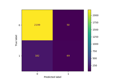
Release Highlights for scikit-learn 1.5
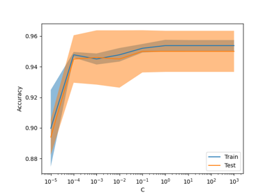
Release Highlights for scikit-learn 1.3
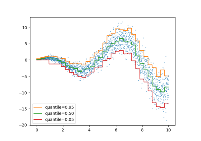
Release Highlights for scikit-learn 1.1

Release Highlights for scikit-learn 1.0
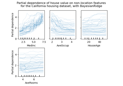
Release Highlights for scikit-learn 0.24
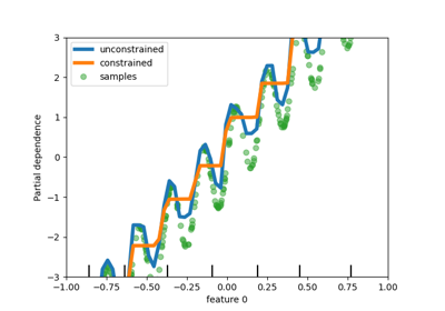
Release Highlights for scikit-learn 0.23
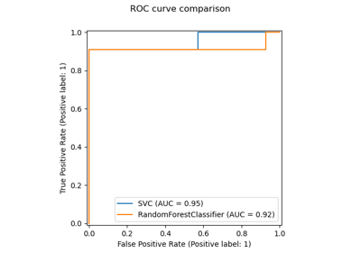
Release Highlights for scikit-learn 0.22
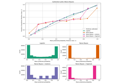
Probability Calibration curves
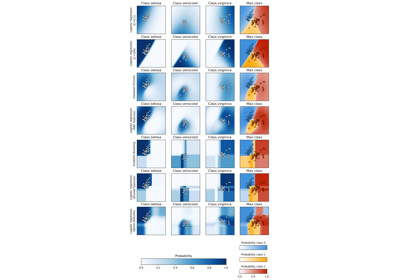
Plot classification probability
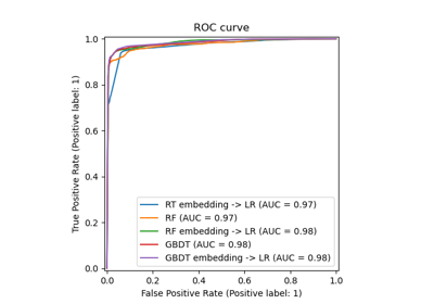
Feature transformations with ensembles of trees
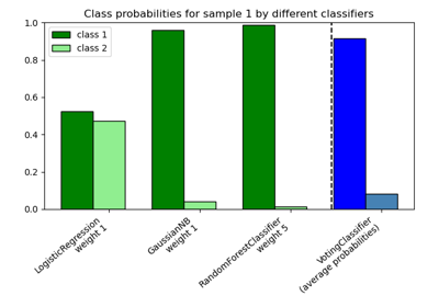
Plot class probabilities calculated by the VotingClassifier
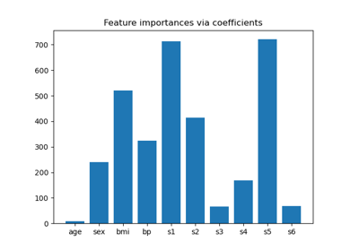
Model-based and sequential feature selection
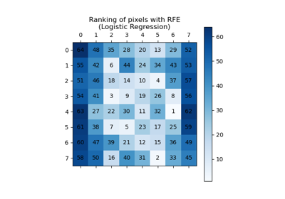
Recursive feature elimination
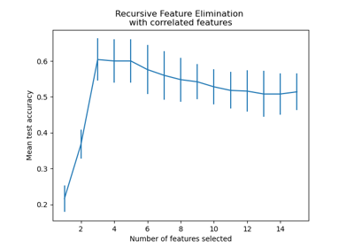
Recursive feature elimination with cross-validation
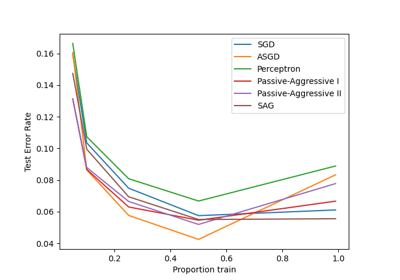
Comparing various online solvers
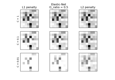
L1 Penalty and Sparsity in Logistic Regression
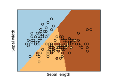
Logistic Regression 3-class Classifier
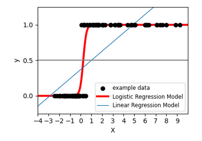
Logistic function
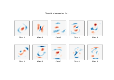
MNIST classification using multinomial logistic + L1
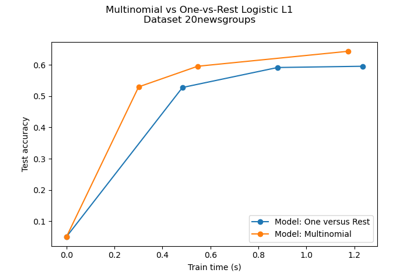
Multiclass sparse logistic regression on 20newgroups
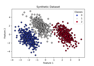
Plot multinomial and One-vs-Rest Logistic Regression
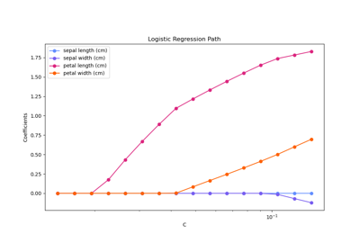
Regularization path of L1- Logistic Regression

Displaying Pipelines

Displaying estimators and complex pipelines
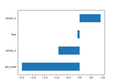
Introducing the set_output API
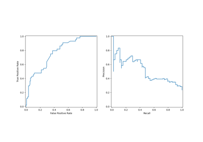
Visualizations with Display Objects
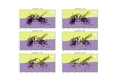
Class Likelihood Ratios to measure classification performance
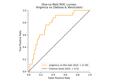
Multiclass Receiver Operating Characteristic (ROC)
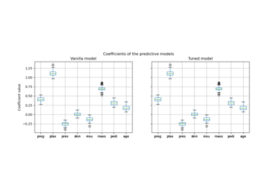
Post-hoc tuning the cut-off point of decision function
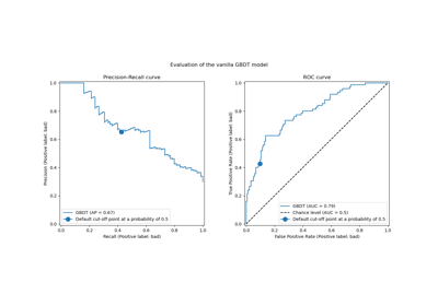
Post-tuning the decision threshold for cost-sensitive learning
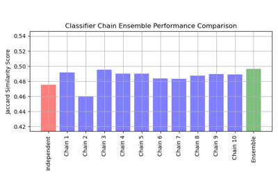
Multilabel classification using a classifier chain
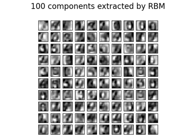
Restricted Boltzmann Machine features for digit classification

Column Transformer with Mixed Types
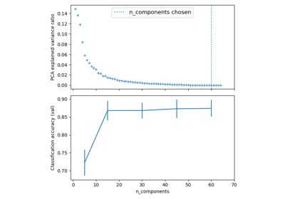
Pipelining: chaining a PCA and a logistic regression
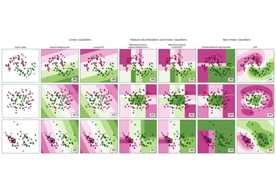
Feature discretization

Digits Classification Exercise
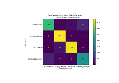
Classification of text documents using sparse features
- Open access
- Published: 26 August 2024
Associations of the planetary health diet index (PHDI) with asthma: the mediating role of body mass index
- Shaoqun Huang 1 na1 ,
- Qiao He 2 na1 ,
- Xiaoxuan Wang 2 ,
- Seok Choi 3 &
- Hongyang Gong 3
BMC Public Health volume 24 , Article number: 2305 ( 2024 ) Cite this article
7 Altmetric
Metrics details
Given the global shifts in environmental conditions and dietary habits, understanding the potential impact of dietary factors and body mass index (BMI) on respiratory diseases, including asthma, is paramount. Investigating these relationships can contribute to the formulation of more effective prevention strategies. The Planetary Health Diet Index (PHDI), a dietary scoring system that balances human health with environmental sustainability, underscores the importance of increasing the consumption of plant-based foods while reducing the intake of red meat, sugar, and highly processed foods. The objective of this study was to assess the association between PHDI and the prevalence of asthma and the mediation effect of BMI in a US general population.
This study utilized data from 32,388 participants in the National Health and Nutrition Examination Survey (NHANES) spanning from 2005 to 2018. Multivariate logistic regression and weighted quantile sum (WQS) regressions were employed to investigate the association between PHDI, individual nutrients, and asthma. Restricted cubic spline (RCS) analysis explored the linear or non-linear relationship between PHDI and asthma. Interaction analyses were conducted on subgroups to validate the findings. Mediation analysis was performed to examine the effect of BMI on the relationship between PHDI and asthma.
There was a significant negative association between PHDI and asthma. After adjusting for covariates, for every 10-point increase in PHDI, there was a 4% decrease in the prevalence of asthma ( P = 0.025). Moreover, as PHDI increased, there was a trend towards lower asthma prevalence (P for trend < 0.05). WQS analyses showed consistent associations (OR = 0.93, 95%CI: 0.88, 0.98), with Fiber, Vitamin C, and Protein significant factors. The dose-response curve indicated a linear association between PHDI and asthma, with higher PHDI associated with lower asthma prevalence. Additionally, BMI is significantly positively associated with asthma ( P < 0.001), and BMI decreases as the PHDI increases (β = -0.64, P < 0.001). Mediation analysis indicates that BMI significantly mediates the relationship between PHDI and asthma, with a mediation proportion of 33.85% ( P < 0.001).
The results of this study show a strong negative correlation between PHDI and the prevalence of asthma. In addition, BMI mediated this negative relationship.
Peer Review reports
Introduction
Asthma is a chronic pulmonary disease and a global health issue affecting individuals of all ages. It is prevalent among both children and adults and is characterized by airway inflammation and muscle tightening, leading to breathing difficulties [ 1 ]. Approximately 350 million people worldwide suffer from asthma [ 2 ], with a prevalence rate of 4.3%. The global crude prevalence is increasing, resulting in 455,000 deaths [ 3 ]. The Global Initiative for Asthma (GINA) predicts that the number of individuals with asthma will reach 400 million by 2025. Prevalence rates vary significantly across countries, with the highest rates observed in developed countries, likely due to aging populations and increased life expectancy [ 4 ]. Asthma is a major cause of severe disability, reduced quality of life, and poor utilization of healthcare resources [ 5 ]. It is a significant contributor to the global burden of non-communicable diseases and is a leading cause of death, second only to cardiovascular diseases and cancer [ 6 ]. Although most asthma patients can achieve control through treatment, the burden of managing the disease remains high, and asthma does not receive as much attention as other non-communicable diseases [ 7 ]. Current strategies for improving asthma prevention are targeted at different risk levels but are not fully utilized. To alleviate the global disease burden and promote universal health, finding effective methods to address this issue is crucial.
Diet is closely related to human health, with approximately 3 billion people worldwide suffering from malnutrition, of which about 2 billion are overnourished. Unhealthy diets increase the burden of diseases on the human body and affect the planet’s carrying capacity, contributing to climate and environmental changes. To better balance the health of humans and the planet, the EAT-Lancet Commission introduced a new dietary metric in 2019—the Planetary Health Diet Index (PHDI) [ 8 ]. The PHDI provides guidelines for various food groups that collectively constitute the optimal diet for human health and environmental sustainability. It emphasizes a higher proportion of plant-based foods, with significant portions of whole grains, fruits, nuts, and vegetables.
The PHDI can potentially prevent 11.6 million premature deaths worldwide, reduce greenhouse gas emissions, decrease environmental pollution, and protect Earth’s biodiversity. Asthma results from the interplay between genetic factors and environmental influences, making it particularly susceptible to climate and environmental changes. Research by Biesbroek S et al. [ 9 ]. indicates that dietary changes in specific contexts depend on the national disease burden (such as obesity or malnutrition), environmental challenges, and cultural traditions. High-income countries, which have a higher risk of chronic non-communicable diseases and a larger environmental footprint, should thus limit consumption. Another longitudinal study involving 1,050 children demonstrated that children living in environments with abundant greenery had a lower risk of developing asthma compared to those born in areas with a higher presence of animals [ 10 ].
Moreover, several studies have shown that a healthy diet may be associated with body mass index (BMI) [ 11 , 12 , 13 ]. BMI, as a proxy for body weight and obesity, is considered closely related to asthma [ 14 , 15 ]. However, whether BMI mediates this relationship remains unknown. Currently, no studies have investigated the association between PHDI and asthma mediated by BMI. For the first time, we investigated the association between the PHDI and asthma prevalence mediated by BMI in this study using a large cross-sectional methodology. It is hypothesized that there may be a negative correlation between the PHDI and asthma prevalence and explored the mediating role of BMI in the correlation between PHDI and asthma prevalence, aiming to validate that an appropriate and healthy PHDI could prevent asthma.
Study population
The National Health and Nutrition Examination Survey (NHANES) is a nationally representative cross-sectional survey conducted through home interviews and mobile examination centers, aimed at assessing the health and nutritional status of the U.S. population. This survey utilized data from 70,190 participants over seven cycles of NHANES, spanning from 2005 to 2018. After excluding individuals younger than 20 years ( n = 30,441), pregnant women ( n = 708), and participants with missing or incomplete PHDI data ( n = 6,653), a total of 32,388 participants were included in the final analysis. Figure 1 displays a flowchart of the entire selection process. NHANES is approved by the Research Ethics Review Board of the National Center for Health Statistics, and all participants provided informed consent. The data used in this study are de-identified and publicly available ( https://www.cdc.gov/nchs/nhanes/index.htm ).

A flow diagram of eligible participant selection in the National Health and Nutrition Examination Survey
Measurement
Planetary health diet index.
The measurement of the PHDI is based on the ranges provided in the EAT-Lancet Commission’s scientific report. It comprises 14 food categories: whole grains, whole fruits, non-starchy vegetables, nuts and seeds, legumes and unsaturated oils, starchy vegetables, dairy products, red and processed meats, poultry, eggs, fish, saturated fats and trans fats, added sugars, and fruit juices. The first six categories are adequacy components that are encouraged for consumption, while the latter eight are moderation components that are discouraged for consumption. Each food category is scored on a scale from 0 to 10, resulting in a theoretical PHDI range from 0 to 140. Further details on the PHDI can be found in previous studies and Table S1 [ 8 , 16 , 17 ].
Diagnosis of asthma
According to previous studies [ 18 , 19 ], the criteria for diagnosing asthma were extracted from the questionnaire section of the NHANES database: (1) “Has a doctor or other health professional ever told you that you have asthma?” (2) “Do you still have asthma?” Participants who answered “yes” to both questions were classified as having asthma, while those who did not were excluded. For a detailed explanation, see the website ( https://www.cdc.gov/nchs/nhanes/index.htm ).
Covariables
We constructed a directed acyclic graph (DAG) [ 20 ] to visualize the hypothesized associations of the primary exposure (Planetary Health Diet Index) with the outcomes of interest (the prevalence of asthma), and potential covariates. According to previous studies [ 21 , 22 , 23 ], the covariates in this research include age, gender, race, marital status, education level, family poverty-to-income ratio (PIR), energy intake, smoking, alcohol consumption, hypertension, diabetes, and hypercholesterolemia. For detailed information on these covariates, please refer to Table S2 . The resulting DAG is presented in Figure S1 .
Statistical analyses
In this study, all data were statistically analyzed using R (version 4.3.1). To guarantee that the data in our investigation were nationally representative, we used the weights that the NCHS suggested. The weighting variable was the two-day dietary sample weight (WTDR2D), and the new weights for the years 2005–2018 were computed as 1/7 × WTDR2D. The data were weighted, with continuous variables presented as mean ± standard deviation, and p-values calculated using weighted Students T-test. Percentages for categorical variables (weighted N, %) and their p-values were calculated using weighted chi-square tests [ 24 ]. The association between PHDI and asthma was analyzed using multivariable logistic regression models, where PHDI was categorized into quartiles. Trend tests and p-values for linear trends were calculated to determine the consistency of the relationship. Three models were constructed in this study: (1) an unadjusted crude model; (2) a model adjusted for age, gender, race, education level, marital status, and family poverty-to-income ratio (PIR); and (3) a model further adjusted for energy intake, smoking, alcohol consumption, hypertension, diabetes, and hypercholesterolemia. A smooth curve fitting was applied to further explore the potential linear relationship between PHDI and asthma. Additionally, odds ratios (ORs) were calculated for every 10-point increase in PHDI, with subgroup analyses conducted based on age, gender, race, marital status, education level, PIR, smoking, alcohol consumption, hypertension, diabetes, and hypercholesterolemia. In the subgroup analysis, we further adjusted for age, gender, race, marital status, education level, PIR, energy intake, smoking, alcohol consumption, hypertension, diabetes, and hypercholesterolemia.
The “mediation” package in R software was used to assess the indirect impact, direct effect, and total effect. A mediation analysis with 1000 bootstrap resamples and correction for variables was carried out to determine if BMI mediated the association between PHDI and asthma. The indirect effect/ (indirect effect + direct effect) ×100% was used to compute the mediated fraction [ 25 ]. The total effect of PHDI on asthma (path C), the direct effect of PHDI on asthma when BMI (mediator) is included in the model (path C′), the effect of PHDI on BMI (path A), the effect of BMI on asthma (path B), and the indirect effect of BMI on the association between PHDI and asthma (path A*B) are all represented by regression coefficients (Figure S2 ).
To evaluate the results obtained in this study from a food science perspective, we added detailed data on the daily consumption of individual nutrients, including energy, carbohydrates, dietary fiber, fats, proteins, vitamins, and minerals, and assessed their impact on asthma. In addition, we applied the weighted quantile sum (WQS) regressions to explore the overall effect of individual single nutrients on asthma. WQS is a new statistical tool for estimating both the collective and specific impacts of exposures [ 26 ]. The data was divided into training sets (40%) and validation sets (60%) at random. The training sets were then bootstrapped 1000 times. We ran the WQS model in the negative direction because metrics had an inverse relationship with asthma. Metric weights varied from 0 to 1 and added up to 1. Major contributors were determined to be the metrics (average of 10 metrics) with weights greater than 0.1. Given that diabetes, hypertension, and hypercholesterolemia can lead to changes in dietary habits, we excluded participants with these conditions and reanalyzed the data (Table S6 ). The significance was determined by p-values below 0.05.
Characteristics of the participants
This study included 32,388 participants, with 52% being female and 48% male. There were 4,618 participants with a history of asthma and 27,770 without. Compared to other racial groups, non-Hispanic whites had a higher incidence of asthma (69%). The prevalence of asthma was higher among participants with at least a high school education (85%). The family poverty-to-income ratio (PIR) was inversely related to asthma prevalence. A higher prevalence of asthma was observed among those who were obese, smoked, consumed alcohol, had hypertension, diabetes, or hypercholesterolemia ( p < 0.05). Participants with the prevalence of asthma had lower PHDI scores ( p < 0.05). Baseline characteristics are detailed in Table 1 .
Relationship between PHDI and asthma
Table 2 of the multivariable logistic regression model demonstrated an association between PHDI and asthma. In model 3, a negative association was found between PHDI and asthma prevalence (OR 0.96, 95% CI 0.92–0.99). This negative association was more pronounced in the higher quartiles of PHDI, specifically Q2 (OR 0.91, 95% CI 0.79–1.05), Q3 (OR 0.89, 95% CI 0.77–0.99), and Q4 (OR 0.86, 95% CI 0.75–0.98), compared to Q1. Trend tests in each model, using Q1 as the reference, also confirmed this finding ( p < 0.05). A smooth curve fitting was employed to assess the association between PHDI and asthma; as shown in Fig. 2 , the correlation between PHDI and asthma was linearly negative (nonlinearity = 0.138).

Dose-response relationships between PHDI and asthma. OR (solid lines) and 95% confidence levels (shaded areas) were adjusted for age, gender, education level, marital, PIR, race, smoking, drinking, energy intake, hypertension, diabetes, and high cholesterol
Subgroup and WQS analysis
The subgroup analysis of the association between PHDI and asthma is shown in Fig. 3 . This analysis explored the stability of the relationship and potential interactions by adjusting and stratifying based on age, gender, education level, marital status, income, race, smoking, alcohol consumption, hypertension, diabetes, and hypercholesterolemia. In the subgroup analysis, no significant interaction was found between PHDI and these stratified variables ( p > 0.05), and the negative correlation remained very stable.

Subgroup analysis between PHDI and asthma. ORs were calculated as per 10 scores increase in PHDI. Analyses were adjusted for age, gender, education level, marital, PIR, race, smoking, drinking, energy intake, hypertension, diabetes, and high cholesterol
In addition, the WQS index from the WQS regression was negatively associated with the risk of asthma (OR 0.93,95% CI 0.88 to 0.98) (Table S5). Figure 4 showed that all nutrients were negatively associated with asthma, with dietary fiber (weight = 0.440) identified as the most important factor influencing the presence of asthma, followed by Vitamin C and Protein (weights = 0.197 and 0.149).

Weights represent the proportion of partial effect for each PHDI metric in the WQS regression. Model adjusted for age, sex, race, PIR, educational level, and marital status
Mediation effect
Table S3 displays the association between BMI and asthma. In model 3, Following adjustment for all covariates, compared to the first quartile (Q1) of BMI, the odds of asthma increased by 44% in the fourth quartile (Q4) [OR = 1.44, 95% CI:1.23, 1.68]. When BMI was considered as a continuous variable, the positive relationship between BMI and asthma remained statistically significant (OR = 1.02, 95% CI: 1.01, 1.03). Following adjustment for all covariates, there was a significant statistical association between PHDI and BMI (β=-0.64, 95% CI: -0.73, -0.56, P < 0.001) (Table S4). Based on the above analysis, our study meets the prerequisites for conducting mediation analysis. Following adjustment for all covariates, we observed the mediation effect of BMI (Figure S2). BMI (indirect effect= -2.36*10 − 3 , P < 0.001; direct effect= -4.70*10 − 3 , P = 0.036) mediated 33.85% (mediation proportion = indirect effect / (indirect effect + direct effect) *100%, P < 0.001) of the association between PHDI and asthma. Therefore, BMI can be considered a mediating factor in the relationship between PHDI and asthma.
Based on the NHANES database, this study found that after adjusting for relevant covariates, there is a negative association between PHDI and the prevalence of asthma and that BMI mediated this relationship, thus validating our hypothesis. The results of the RCS and subgroup analyses reaffirmed that higher PHDI scores are beneficial in reducing the prevalence of asthma. Additionally, WQS analysis suggests that dietary components of the PHD, including fiber, vitamin C, and protein, play significant roles in the development of asthma.
An important pathogenic mechanism of asthma is airway hyperresponsiveness. Upon exposure to allergens, various inflammatory cells such as eosinophils, mast cells, T cells, neutrophils, airway epithelial cells, and macrophages release inflammatory mediators and cytokines. This release causes damage to airway epithelial cells and exposes epithelial nerve endings, leading to hyperresponsiveness. Studies [ 27 ] indicate that the underlying mechanisms of asthma are multifactorial, involving environmental factors, genetic predispositions, and lifestyle choices, with diet being a significant factor. Previous research [ 28 ] has found a positive correlation between asthma prevalence and gross domestic product (GDP). For instance, the prevalence of asthma in developed Western countries is typically around 10%, whereas in less developed countries, it is ≤ 1% [ 29 ].
The disparity in asthma prevalence between developed and developing countries can be attributed not only to underdiagnosis, high misdiagnosis rates, and inadequate treatment in low- and middle-income countries but also to differences in dietary patterns. Studies [ 30 ] have shown that Western dietary patterns emphasize animal-based foods while neglecting whole grains, fruits, vegetables, and legumes. For example, the intake of saturated fats in the U.S. population, which follows a predominantly Western diet, significantly exceeds recommended levels, while fruit and vegetable consumption falls below the norm. As dietary patterns westernize, the risk of asthma increases [ 31 ]. In contrast, diets that emphasize whole grains, fruits, vegetables, and legumes, and de-emphasize high-fat meats and dairy products, are beneficial in reducing asthma risk. A case-control study involving 287 children aged 9–19 in Lima, Peru [ 32 ], used a modified Mediterranean Diet Score (MDS) to analyze dietary patterns. Preliminary analysis showed a negative correlation between adherence to the Mediterranean diet and the incidence of asthma in children. Similar plant-based dietary patterns have also been shown to reduce asthma risk [ 33 , 34 ]. A meta-analysis and systematic review of 31 studies evaluated asthma outcomes such as prevalence, asthma-related quality of life, symptoms, lung function, frequency of asthma attacks, asthma control, and inflammatory markers associated with asthma. The results indicated a significant association between dietary patterns and asthma in 12 of the studies, with protective dietary patterns including components like black bread, nuts, and wine [ 35 ]. Adhering to a plant-based dietary pattern can result in higher PHDI scores. A multicenter cohort study conducted in Brazil with 14,779 participants using a 114-item Food Frequency Questionnaire (FFQ) found that the PHDI was positively correlated with carbohydrates, plant proteins, polyunsaturated fats, fiber, and micronutrients from fruits, vegetables, oilseeds, and whole grains. In the PHDI, nuts and peanuts, legumes, fruits, total vegetables, and whole grains are defined as adequacy components. Recent research [ 36 ] showed that PHDI scores are positively correlated with plant protein, fiber, polyunsaturated fats, vitamins A, E, K, C, and folic acid ( p < 0.001), and negatively correlated with animal protein, total fat, monounsaturated fats, and riboflavin ( p < 0.001).
This study indicates that dietary fiber, vitamin C, and protein play significant roles in the development of asthma. Meta-analyses [ 37 ] have long shown that high consumption of fruits and vegetables is associated with a reduced risk of asthma in both children and adults. Retrospective studies [ 38 ] have demonstrated that a high intake of fruits and vegetables is correlated with higher forced expiratory volume in one second (FEV1), reducing the risk of asthma and the incidence of wheezing. Fruit and vegetable consumption can also effectively control and alleviate symptoms during asthma attacks. A cohort study involving 2,870 children [ 39 ] showed that habitual fruit consumption helps alleviate asthma symptoms (OR = 0.93, 95% CI 0.85-1.00), and long-term fruit intake was negatively correlated with the frequency of asthma symptoms (OR = 0.90, 95% CI 0.82–0.99) and allergen sensitization (OR = 0.90, 95% CI 0.82–0.99). However, Willers et al. further noted that increased consumption of certain foods, whether early or late in life or over extended periods, does not have a consistent impact on asthma and atopy in 8-year-old children [ 39 ]. Consequently, fruit intake may be inversely related to asthma. A prospective cohort study [ 40 ] observing 520 children found that fruit intake was inversely associated with the incidence of asthma, rhinitis, and allergy symptoms. The incidence of asthma symptoms decreased from 33.3 to 28.3% to 14.3% across groups with increasing fruit intake (P for trend = 0.01). Additionally, a Dutch study indicated a negative correlation between whole grain consumption and asthma incidence, which our study further supports.
Whole grains are essential components of a healthy diet, providing dietary fiber, B vitamins, minerals, and other nutrients. Early epidemiological studies have linked asthma prevalence to dietary habits. A study using questionnaires and clinical data to define asthma [ 41 ] found a negative correlation between whole grain intake and asthma (OR = 0.46, 95% CI 0.19-10), suggesting that high consumption of whole grain products may reduce asthma attacks in children. A Danish study [ 42 ] used a disease-death multi-state model to evaluate the correlation between whole grain intake and life expectancy (defined as 20 years of follow-up without cancer, asthma, chronic obstructive pulmonary disease, etc.). It found that for every doubling of whole grain intake, the difference in disease-free life expectancy (without cancer, type 2 diabetes, ischemic heart disease, stroke, asthma, chronic obstructive pulmonary disease or dementia or with disease (any of the listed)) increased by 0.43 (95% CI: 0.33–0.52) in men and 0.15 (95% CI: 0.06–0.24) in women over an average follow-up period of 13.8 and 17.5 years for 22,606 men and 25,468 women, respectively. Furthermore, studies have shown that dietary fiber intake is positively correlated with improved lung function. Higher fiber intake was associated with higher average FEV1 and FVC measurements, with those consuming the most fiber having average FEV1 and FVC values that were 82 ml and 129 ml higher than those consuming the least fiber ( P = 0.05 and 0.01, respectively). Therefore, a fiber-rich diet may also play a role in improving asthma [ 43 ].
Current observational and clinical research evidence suggests that plant-based dietary patterns (primarily consisting of fruits, vegetables, and whole grains) are valuable in preventing asthma, whereas Western dietary patterns (emphasizing red meat, processed meats, refined grains, and added sugars) appear to increase asthma risk [ 44 ]. As a modifiable factor affecting lung health [ 45 ], the protective effects of a plant-based dietary model (corresponding to higher PHDI scores) may be associated with oxidative stress, inflammation, and gut microbiota. In contrast, the exacerbation of asthma by a Western dietary model (corresponding to lower PHDI scores) is likely linked to inflammation.
Oxidative stress and inflammation are key mechanisms by which diet influences asthma. Oxidative stress occurs when the balance between the production and elimination of free radicals is disrupted, leading to neutrophilic inflammatory infiltration and increased secretion of proteases, resulting in the production of a large amount of reactive oxygen species (ROS). Excessive ROS can also increase the expression of NLRP3, triggering the release of pro-inflammatory cytokines and inducing inflammation. During inflammation, mast cells and leukocytes accumulate at the damaged site, increasing oxygen intake and subsequently the release and accumulation of ROS at the site, thereby exacerbating oxidative stress. Oxidative stress and inflammation are associated with poor asthma outcomes. When the lungs are exposed to oxidative stress and an inflammatory environment, it can lead to pulmonary dysfunction such as asthma. Research by Wood LG et al. [ 46 , 47 ]. confirmed that a diet rich in plant-based foods (high PHDI scores) can reduce inflammatory responses and enhance anti-inflammatory factors. Early studies [ 48 ] have shown that adopting a plant-based diet provides antioxidants and unsaturated fatty acids, which can alleviate oxidative stress and inflammation, thus mitigating asthma. Increased intake of fruits and vegetables is negatively correlated with the number of pro-inflammatory cytokines and airway neutrophils in asthma patients [ 49 ]. Whole grains also have antioxidant and anti-inflammatory properties. Studies [ 50 ] have shown that higher consumption of whole grains is associated with lower levels of serum C-reactive protein and tumor necrosis factor-α receptor-2. Conversely, Western dietary patterns exacerbate oxidative stress and inflammation. Research [ 51 ] indicates that dairy consumption is positively correlated with the concentration of pro-inflammatory interleukin (IL)-17 F ( P < 0.05), suggesting that the IL-17 F-dependent inflammatory pathway may mediate asthma development. Kim et al. [ 52 ]. found that a high-fat diet induces the production of numerous pulmonary cytokines, increasing airway hyperresponsiveness and inflammation, as evidenced by elevated IL-6 and IL-8 expression in sputum samples. A diet high in mixed fats not only increases the release of TNF-α and IL-6 but also activates Toll-like receptors, triggering immune responses [ 53 ].
The composition and function of respiratory and gut microbiota interact, known as the “gut-lung axis,” and are related to airway immune function. Dysfunction of the airway epithelial barrier and increased permeability contribute to antigen sensitization and the progression of asthma. Concurrently, gut microbiota dysbiosis can increase the risk of asthma. Gut microbiota is closely related to dietary patterns, with different diets influencing the production of various metabolites by gut microbiota, thereby affecting immune responses and modulating pulmonary pro-inflammatory reactions [ 54 ]. Studies have shown that plant-based diets (with high PHDI scores) can modulate gut immune responses to improve airway inflammation [ 55 ]. Intake of dietary fiber can lead to the production of short-chain fatty acids by gut microbiota, which have a regulatory effect on immune responses. Consuming yogurt can supplement the body with prebiotics, which are dietary supplements that regulate gut microbiota, affect blood lipid levels, and enhance immune system function. Research [ 56 ] indicates that women who take prebiotics during pregnancy and lactation may reduce the risk of allergen sensitization.
This study found that BMI mediates the association between PHDI and asthma, potentially through the following mechanisms: (1) The dietary patterns within PHDI may influence asthma risk through their impact on BMI. For instance, diets rich in vegetables, fruits, and whole grains help maintain a healthy BMI [ 57 ], potentially reducing asthma risk. Conversely, high-fat and high-sugar diets may increase BMI [ 58 ], thereby elevating asthma risk. (2) The gut microbiota in obese individuals typically differs significantly from that of healthy individuals, often characterized by a reduction in beneficial bacteria and an increase in harmful bacteria [ 59 ]. This dysbiosis can affect lung health via the “gut-lung axis,” increasing airway susceptibility [ 54 ]. Elevated BMI may mediate the relationship between PHDI and asthma indirectly by altering gut microbiota composition, particularly when high-fat and high-sugar diets further disrupt the gut microbiome. (3) Increased BMI may influence immune system function [ 60 ], potentially affecting how certain dietary components in PHDI (such as high sugar or high fat) impact asthma risk through BMI’s effects on the immune system. (4) Individuals with higher BMI are more likely to experience airway narrowing and airflow limitation [ 61 ], which may increase susceptibility to asthma or exacerbate asthma symptoms during an attack. The mechanical pressure of obesity on the airways could amplify the effects of unhealthy diets within PHDI. (5) Expansion of adipose tissue in obese individuals leads to macrophage infiltration and elevated levels of pro-inflammatory cytokines (e.g., TNF-α, IL-6, and CRP) [ 62 ]. These inflammatory markers can affect the lungs via the bloodstream, increasing airway inflammation and thereby worsening or triggering asthma symptoms [ 63 ]. Elevated BMI may enhance or accelerate the negative impact of unhealthy dietary components in PHDI on asthma risk through this systemic inflammation pathway.
In summary, the PHDI is a dietary metric representing both planetary and human dietary health. Asthma, beyond its genetic predispositions, is closely associated with diet and environmental factors. Current research predominantly focuses on the relationships between dietary patterns, dietary fiber, and nutrients with asthma. There has been no previous research on the association between PHDI and asthma risk in adults. This study is the first to investigate the role of BMI in the relationship between PHDI and asthma prevalence using the NHANES database. First, a multivariable logistic regression model demonstrated a negative correlation between PHDI and asthma. Smooth curve fitting assessed the relationship, confirming a negative and linear correlation (nonlinearity = 0.138). Subgroup analyses adjusting for age, gender, education level, marital status, income, race, energy intake, smoking, alcohol consumption, hypertension, diabetes, and hypercholesterolemia showed no significant interaction between PHDI and these stratified variables ( p > 0.05), indicating a very stable relationship. Finally, the mediation analysis results indicate that BMI serves as a mediator in the association between PHDI and asthma. Literature review reveals that plant-based dietary patterns correspond to higher PHDI scores, while Western and high-fat dietary patterns correspond to lower PHDI scores. Previous studies have found that a high intake of fruits, vegetables, and grains can reduce the risk of asthma [ 37 , 38 ], whereas a high intake of red meat, eggs, fish, saturated fats trans fats, added sugars and fruit juices increases the risk of asthma. The underlying mechanisms are closely related to oxidative stress, inflammation, and gut microbiota.
Additionally, this study has limitations: (1) The cross-sectional nature of the data limits causal inference, and although PHDI may have an impact on asthma through BMI, more comprehensive prospective cohort studies, randomized controlled trials, or animal studies are required in the future to determine the precise pathogenic processes. (2) The constraints of the NHANES database preclude us from eliminating the potential confounding factors’ ultimate impact on the study results, even though we included a reasonably high number of covariates based on prior research to improve the robustness of our study results. As a result, it is important to interpret the study’s findings carefully and impartially. (3) Given that the analysis of the relationship between dietary components and disease risk should adhere to the isocaloric principle, incorporating all macronutrients, micronutrients, and energy within the same model may introduce bias [ 64 ]. Consequently, the WQS analysis results in this study should be interpreted with caution. (4) The development of the PHDI is based on the Food Frequency Questionnaire (FFQ). Although the FFQ is the most used method in epidemiological studies to investigate the relationship between diet and health outcomes, it has its limitations. These include the incompleteness of the food list and the potential for recall bias in the reports provided [ 65 ]. (5) It is well known that asthma is associated with socioeconomic status, urbanization, and local air pollution levels, all of which play a significant role in the pathogenesis of asthma [ 66 ]. In the future, we plan to pursue multicenter studies with larger sample sizes or explore alternative study designs to address this limitation.
In conclusion, our study indicates a linear inverse association between PHDI and asthma risk, with BMI mediating this relationship. Randomized controlled trials are necessary to further explore the connection between PHDI and asthma symptoms. Future prospective studies and fundamental experiments are needed to delve deeper into the mechanisms, which can then guide dietary recommendations for asthma patients while promoting both planetary and human health. Providing specific dietary structure recommendations can offer new perspectives for the comprehensive prevention and treatment of chronic non-communicable diseases like asthma, thus reducing the global disease burden. Integrating human dietary health, respiratory health, and planetary health into a unified approach can advance universal health coverage and alleviate the global disease burden.
Data availability
The study involved the analysis of publicly available datasets. The data can be accessed at the following URL: https://www.cdc.gov/nchs/nhanes/.
GBD 2019 Diseases and Injuries Collaborators. Global burden of 369 diseases and injuries in 204 countries and territories, 1990–2019: a systematic analysis for the global burden of Disease Study 2019. Lancet. 2020;396:1204–22.
Article Google Scholar
García-Marcos L, Chiang C-Y, Asher MI, Marks GB, El Sony A, Masekela R, et al. Asthma management and control in children, adolescents, and adults in 25 countries: a global Asthma Network Phase I cross-sectional study. Lancet Glob Health. 2023;11:e218–28.
Article PubMed PubMed Central Google Scholar
Papi A, Brightling C, Pedersen SE, Reddel HK, Asthma. Lancet. 2018;391:783–800.
Article PubMed Google Scholar
To T, Stanojevic S, Moores G, Gershon AS, Bateman ED, Cruz AA, et al. Global asthma prevalence in adults: findings from the cross-sectional world health survey. BMC Public Health. 2012;12:204.
Raghavan D, Jain R. Increasing awareness of sex differences in airway diseases. Respirology. 2016;21:449–59.
GBD Chronic Respiratory Disease Collaborators. Prevalence and attributable health burden of chronic respiratory diseases, 1990–2017: a systematic analysis for the global burden of Disease Study 2017. Lancet Respir Med. 2020;8:585–96.
GBD 2015 Chronic Respiratory Disease Collaborators. Global, regional, and national deaths, prevalence, disability-adjusted life years, and years lived with disability for chronic obstructive pulmonary disease and asthma, 1990–2015: a systematic analysis for the global burden of Disease Study 2015. Lancet Respir Med. 2017;5:691–706.
Willett W, Rockström J, Loken B, Springmann M, Lang T, Vermeulen S, et al. Food in the Anthropocene: the EAT-Lancet Commission on healthy diets from sustainable food systems. Lancet. 2019;393:447–92.
Biesbroek S, Kok FJ, Tufford AR, Bloem MW, Darmon N, Drewnowski A, et al. Toward healthy and sustainable diets for the 21st century: importance of sociocultural and economic considerations. Proc Natl Acad Sci U S A. 2023;120:e2219272120.
Cavaleiro Rufo J, Paciência I, Hoffimann E, Moreira A, Barros H, Ribeiro AI. The neighbourhood natural environment is associated with asthma in children: a birth cohort study. Allergy. 2021;76:348–58.
Gutiérrez-Pliego LE, Camarillo-Romero E, del Montenegro-Morales S, de Garduño-García LP. J. Dietary patterns associated with body mass index (BMI) and lifestyle in Mexican adolescents. BMC Public Health. 2016;16:850.
Platikanova M, Yordanova A, Hristova P. Dependence of body Mass Index on some Dietary habits: an application of classification and regression tree. Iran J Public Health. 2022;51:1283–94.
PubMed PubMed Central Google Scholar
Newby P, Muller D, Hallfrisch J, Qiao N, Andres R, Tucker KL. Dietary patterns and changes in body mass index and waist circumference in adults123. Am J Clin Nutr. 2003;77:1417–25.
Kang M, Sohn S-J, Shin M-H. Association between Body Mass Index and Prevalence of Asthma in Korean adults. Chonnam Med J. 2020;56:62–7.
Hjellvik V, Tverdal A, Furu K. Body mass index as predictor for asthma: a cohort study of 118,723 males and females. Eur Respir J. 2010;35:1235–42.
Frank SM, Jaacks LM, Adair LS, Avery CL, Meyer K, Rose D, et al. Adherence to the Planetary Health Diet Index and correlation with nutrients of public health concern: an analysis of NHANES 2003–2018. Am J Clin Nutr. 2024;119:384–92.
Frank SM, Jaacks LM, Meyer K, Rose D, Adair LS, Avery CL, et al. Dietary quality and dietary greenhouse gas emissions in the USA: a comparison of the planetary health diet index, healthy eating index-2015, and dietary approaches to stop hypertension. Int J Behav Nutr Phys Act. 2024;21:36.
Tian Z, Li X, Han Y, Zhang X. The association between the composite dietary antioxidant index and asthma in US children aged 3–18 years: a cross-sectional study from NHANES. Sci Rep. 2024;14:17204.
Wang K, Chen Z, Wei Z, He L, Gong L. Association between body fat distribution and asthma in adults: results from the cross-sectional and bidirectional mendelian randomization study. Front Nutr. 2024;11:1432973.
Li Y, Liu X, Lv W, Wang X, Du Z, Liu X, et al. Metformin use correlated with lower risk of cardiometabolic diseases and related mortality among US cancer survivors: evidence from a nationally representative cohort study. BMC Med. 2024;22:269.
Wang Y, Han X, Li J, Zhang L, Liu Y, Jin R, et al. Associations between the compositional patterns of blood volatile organic compounds and chronic respiratory diseases and ages at onset in NHANES 2003–2012. Chemosphere. 2023;327:138425.
Sveiven SN, Bookman R, Ma J, Lyden E, Hanson C, Nordgren TM. Milk consumption and respiratory function in Asthma patients: NHANES Analysis 2007–2012. Nutrients. 2021;13:1182.
Cheng W, Bu X, Xu C, Wen G, Kong F, Pan H, et al. Higher systemic immune-inflammation index and systemic inflammation response index levels are associated with stroke prevalence in the asthmatic population: a cross-sectional analysis of the NHANES 1999–2018. Front Immunol. 2023;14:1191130.
Feng G, Huang S, Zhao W, Gong H. Association between life’s essential 8 and overactive bladder. Sci Rep. 2024;14:11842.
Wang S, Shan T, Zhu J, Jiang Q, Gu L, Sun J, et al. Mediation effect of body Mass Index on the Association of Urinary Nickel Exposure with serum lipid profiles. Biol Trace Elem Res. 2023;201:2733–43.
Zhao S, Tang Y, Li Y, Shen H, Liu A. Associations between Life’s essential 8 and depression among US adults. Psychiatry Res. 2024;338:115986.
Wen J, Wang C, Giri M, Guo S. Association between serum folate levels and blood eosinophil counts in American adults with asthma: results from NHANES 2011–2018. Front Immunol. 2023;14:1134621.
Wang D, Xiao W, Ma D, Zhang Y, Wang Q, Wang C, et al. Cross-sectional epidemiological survey of asthma in Jinan, China. Respirology. 2013;18:313–22.
Paciência I, Cavaleiro Rufo J. Urban-level environmental factors related to pediatric asthma. Porto Biomed J. 2020;5:e57.
Kim J-H, Ellwood PE, Asher MI. Diet and Asthma: looking back, moving forward. Respir Res. 2009;10:49.
Lee-Kwan SH, Moore LV, Blanck HM, Harris DM, Galuska D. Disparities in State-Specific Adult Fruit and Vegetable Consumption - United States, 2015. MMWR Morb Mortal Wkly Rep. 2017;66:1241–7.
Rice JL, Romero KM, Galvez Davila RM, Meza CT, Bilderback A, Williams DL, et al. Association between Adherence to the Mediterranean Diet and Asthma in Peruvian children. Lung. 2015;193:893–9.
Vassilopoulou E, Guibas GV, Papadopoulos NG. Mediterranean-Type diets as a protective factor for Asthma and Atopy. Nutrients. 2022;14:1825.
Bédard A, Northstone K, Henderson AJ, Shaheen SO. Mediterranean diet during pregnancy and childhood respiratory and atopic outcomes: birth cohort study. Eur Respir J. 2020;55:1901215.
Lv N, Xiao L, Ma J. Dietary pattern and asthma: a systematic review and meta-analysis. J Asthma Allergy. 2014;7:105–21.
Cacau LT, De Carli E, de Carvalho AM, Lotufo PA, Moreno LA, Bensenor IM, et al. Development and validation of an Index based on EAT-Lancet recommendations: the Planetary Health Diet Index. Nutrients. 2021;13:1698.
Uddenfeldt M, Janson C, Lampa E, Leander M, Norbäck D, Larsson L, et al. High BMI is related to higher incidence of asthma, while a fish and fruit diet is related to a lower- results from a long-term follow-up study of three age groups in Sweden. Respir Med. 2010;104:972–80.
Mendes F, de Paciência C, Cavaleiro Rufo I, Farraia J, Silva M, Padrão D. Higher diversity of vegetable consumption is associated with less airway inflammation and prevalence of asthma in school-aged children. Pediatr Allergy Immunol. 2021;32:925–36.
Willers SM, Wijga AH, Brunekreef B, Scholtens S, Postma DS, Kerkhof M, et al. Childhood diet and asthma and atopy at 8 years of age: the PIAMA birth cohort study. Eur Respir J. 2011;37:1060–7.
Kusunoki T, Takeuchi J, Morimoto T, Sakuma M, Yasumi T, Nishikomori R, et al. Fruit intake reduces the onset of respiratory allergic symptoms in schoolchildren. Pediatr Allergy Immunol. 2017;28:793–800.
Tabak C, Wijga AH, de Meer G, Janssen N, a. H, Brunekreef B, Smit HA. Diet and Asthma in Dutch school children (ISAAC-2). Thorax. 2006;61:1048–53.
Eriksen AK, Grand MK, Kyrø C, Wohlfahrt J, Overvad K, Tjønneland A, et al. Whole-grain intake in mid-life and healthy ageing in the Danish Diet, Cancer and Health cohort. Eur J Nutr. 2024. https://doi.org/10.1007/s00394-024-03357-3 .
Hanson C, Lyden E, Rennard S, Mannino DM, Rutten EPA, Hopkins R, et al. The relationship between Dietary Fiber intake and lung function in the National Health and Nutrition Examination Surveys. Ann Am Thorac Soc. 2016;13:643–50.
Medina-Remón A, Kirwan R, Lamuela-Raventós RM, Estruch R. Dietary patterns and the risk of obesity, type 2 diabetes mellitus, cardiovascular diseases, asthma, and neurodegenerative diseases. Crit Rev Food Sci Nutr. 2018;58:262–96.
Visser E, de Jong K, van Zutphen T, Kerstjens HAM, Ten Brinke A. Dietary inflammatory index and clinical outcome measures in adults with moderate-to-severe asthma. J Allergy Clin Immunol Pract. 2023;11:3680–e36897.
Wood LG, Baines KJ, Fu J, Scott HA, Gibson PG. The neutrophilic inflammatory phenotype is associated with systemic inflammation in asthma. Chest. 2012;142:86–93.
Fu J, Baines KJ, Wood LG, Gibson PG. Systemic inflammation is associated with differential gene expression and airway neutrophilia in asthma. OMICS. 2013;17:187–99.
Schwingshackl L, Hoffmann G. Mediterranean dietary pattern, inflammation and endothelial function: a systematic review and meta-analysis of intervention trials. Nutr Metab Cardiovasc Dis. 2014;24:929–39.
Wood LG, Garg ML, Smart JM, Scott HA, Barker D, Gibson PG. Manipulating antioxidant intake in asthma: a randomized controlled trial. Am J Clin Nutr. 2012;96:534–43.
Slavin JL, Jacobs D, Marquart L, Wiemer K. The role of whole grains in disease prevention. J Am Diet Assoc. 2001;101:780–5.
Han Y-Y, Forno E, Brehm JM, Acosta-Pérez E, Alvarez M, Colón-Semidey A, et al. Diet, interleukin-17, and childhood asthma in Puerto ricans. Ann Allergy Asthma Immunol. 2015;115:288–e2931.
Kim HY, Lee HJ, Chang Y-J, Pichavant M, Shore SA, Fitzgerald KA, et al. Interleukin-17-producing innate lymphoid cells and the NLRP3 inflammasome facilitate obesity-associated airway hyperreactivity. Nat Med. 2014;20:54–61.
Simpson JL, Grissell TV, Douwes J, Scott RJ, Boyle MJ, Gibson PG. Innate immune activation in neutrophilic asthma and bronchiectasis. Thorax. 2007;62:211–8.
Alwarith J, Kahleova H, Crosby L, Brooks A, Brandon L, Levin SM, et al. The role of nutrition in asthma prevention and treatment. Nutr Rev. 2020;78:928–38.
Vutcovici M, Brassard P, Bitton A. Inflammatory bowel disease and airway diseases. World J Gastroenterol. 2016;22:7735–41.
Adjibade M, Vigneron L, Delvert R, Adel-Patient K, Divaret-Chauveau A, Annesi-Maesano I et al. Characteristics of infant formula consumed in the first months of life and allergy in the EDEN mother-child cohort. Matern Child Nutr. 2024;:e13673.
Mellendick K, Shanahan L, Wideman L, Calkins S, Keane S, Lovelady C. Diets Rich in Fruits and vegetables are Associated with Lower Cardiovascular Disease Risk in adolescents. Nutrients. 2018;10:136.
Moreno-Fernández S, Garcés-Rimón M, Vera G, Astier J, Landrier JF, Miguel M. High Fat/High glucose Diet induces metabolic syndrome in an experimental rat model. Nutrients. 2018;10:1502.
Liu B-N, Liu X-T, Liang Z-H, Wang J-H. Gut microbiota in obesity. World J Gastroenterol. 2021;27:3837–50.
Morąg B, Kozubek P, Gomułka K. Obesity and selected allergic and immunological Diseases—Etiopathogenesis, Course and Management. Nutrients. 2023;15:3813.
Franssen FM. Obesity, airflow limitation, and respiratory symptoms: does it take three to tango? Prim Care Respir J. 2012;21:131–3.
Kunz HE, Hart CR, Gries KJ, Parvizi M, Laurenti M, Dalla Man C, et al. Adipose tissue macrophage populations and inflammation are associated with systemic inflammation and insulin resistance in obesity. Am J Physiol Endocrinol Metab. 2021;321:E105–21.
Canöz M, Erdenen F, Uzun H, Müderrisoglu C, Aydin S. The relationship of inflammatory cytokines with asthma and obesity. Clin Invest Med. 2008;31:E373–379.
Willett WC, Howe GR, Kushi LH. Adjustment for total energy intake in epidemiologic studies. Am J Clin Nutr. 1997;65 4 Suppl:1220S-1228S; discussion 1229S-1231S.
Thompson FE, Kirkpatrick SI, Subar AF, Reedy J, Schap TE, Wilson MM, et al. The National Cancer Institute’s Dietary Assessment primer: a resource for Diet Research. J Acad Nutr Diet. 2015;115:1986–95.
Asthma. https://www.who.int/news-room/fact-sheets/detail/asthma . Accessed 18 Aug 2024.
Download references
Acknowledgements
We are very grateful to the NHANES database for all the data provided.
This study was not financially supported by any governmental, corporate, or non-profit entities.
Author information
Shaoqun Huang, Qiao He contributed equally to this work.
Authors and Affiliations
Department of Oncology Surgery, Fuzhou Hospital of Traditional Chinese Medicine Affiliated to Fujian University of Traditional Chinese Medicine, Fuzhou City, Fujian Province, China
Shaoqun Huang
Graduate School of Tianjin, University of Traditional Chinese Medicine, Tianjin City, China
Qiao He & Xiaoxuan Wang
Department of Physiology, College of Medicine, Chosun University, Gwangju, Korea
Seok Choi & Hongyang Gong
You can also search for this author in PubMed Google Scholar
Contributions
S.H. contributed to the original draft, Methodology, Supervision, Project administration, and Formal analysis. Q.H. contributed to the original draft, Methodology, and Formal analysis. X.W. contributed to Conceptualization, Methodology, Validation, Formal analysis, Resources, and Data curation. S.C. contributed to Validation, Formal analysis, Resources, and Data curation. H.G. was involved in Writing – review & editing, Supervision, Project administration, and Investigation.
Corresponding author
Correspondence to Hongyang Gong .
Ethics declarations
Ethics approval and consent to participate.
Data survey conducted by NHANES has been approved by the NCHS Research Ethics Review Board (ERB). All information from the NHANES program is available and free for public, so an individual investigator was not necessary to obtain approval from the institution’s internal ethics review board.
Consent for publication
Not Applicable.
Competing interests
The authors declare no competing interests.
Additional information
Publisher’s note.
Springer Nature remains neutral with regard to jurisdictional claims in published maps and institutional affiliations.
Electronic supplementary material
Below is the link to the electronic supplementary material.
Supplementary Material 1
Rights and permissions.
Open Access This article is licensed under a Creative Commons Attribution-NonCommercial-NoDerivatives 4.0 International License, which permits any non-commercial use, sharing, distribution and reproduction in any medium or format, as long as you give appropriate credit to the original author(s) and the source, provide a link to the Creative Commons licence, and indicate if you modified the licensed material. You do not have permission under this licence to share adapted material derived from this article or parts of it. The images or other third party material in this article are included in the article’s Creative Commons licence, unless indicated otherwise in a credit line to the material. If material is not included in the article’s Creative Commons licence and your intended use is not permitted by statutory regulation or exceeds the permitted use, you will need to obtain permission directly from the copyright holder. To view a copy of this licence, visit http://creativecommons.org/licenses/by-nc-nd/4.0/ .
Reprints and permissions
About this article
Cite this article.
Huang, S., He, Q., Wang, X. et al. Associations of the planetary health diet index (PHDI) with asthma: the mediating role of body mass index. BMC Public Health 24 , 2305 (2024). https://doi.org/10.1186/s12889-024-19856-1
Download citation
Received : 10 July 2024
Accepted : 22 August 2024
Published : 26 August 2024
DOI : https://doi.org/10.1186/s12889-024-19856-1
Share this article
Anyone you share the following link with will be able to read this content:
Sorry, a shareable link is not currently available for this article.
Provided by the Springer Nature SharedIt content-sharing initiative
- Planetary Health Diet Index
- Mediation analysis
- Body mass index
BMC Public Health
ISSN: 1471-2458
- General enquiries: [email protected]
IMAGES
COMMENTS
The formula on the right side of the equation predicts the log odds of the response variable taking on a value of 1. Simple logistic regression uses the following null and alternative hypotheses: H0: β1 = 0. HA: β1 ≠ 0. The null hypothesis states that the coefficient β1 is equal to zero.
Testing a single logistic regression coefficient in R To test a single logistic regression coefficient, we will use the Wald test, βˆ j −β j0 seˆ(βˆ) ∼ N(0,1), where seˆ(βˆ) is calculated by taking the inverse of the estimated information matrix. This value is given to you in the R output for β j0 = 0. As in linear regression ...
12.1 - Logistic Regression. Logistic regression models a relationship between predictor variables and a categorical response variable. For example, we could use logistic regression to model the relationship between various measurements of a manufactured specimen (such as dimensions and chemical composition) to predict if a crack greater than 10 ...
The logistic regression classifier will predict "Male" if: This is because the logistic regression " threshold " is set at g (z)=0.5, see the plot of the logistic regression function above for verification. For our data set the values of θ are: To get access to the θ parameters computed by scikit-learn one can do: # For theta_0: print ...
In regression analysis, logistic regression[ 1] (or logit regression) estimates the parameters of a logistic model (the coefficients in the linear or non linear combinations). In binary logistic regression there is a single binary dependent variable, coded by an indicator variable, where the two values are labeled "0" and "1", while the ...
Linear Regression VS Logistic Regression Graph| Image: Data Camp. We can call a Logistic Regression a Linear Regression model but the Logistic Regression uses a more complex cost function, this cost function can be defined as the 'Sigmoid function' or also known as the 'logistic function' instead of a linear function. The hypothesis of logistic regression tends it to limit the cost ...
Logistic Function (Image by author) Hence the name logistic regression. This logistic function is a simple strategy to map the linear combination "z", lying in the (-inf,inf) range to the probability interval of [0,1] (in the context of logistic regression, this z will be called the log(odd) or logit or log(p/1-p)) (see the above plot). ). Consequently, Logistic regression is a type of ...
logistic (or logit) transformation, log p 1−p. We can make this a linear func-tion of x without fear of nonsensical results. (Of course the results could still happen to be wrong, but they're not guaranteed to be wrong.) This last alternative is logistic regression. Formally, the model logistic regression model is that log p(x) 1− p(x ...
Logistic Regression. Logistic regression is a GLM used to model a binary categorical variable using numerical and categorical predictors. We assume a binomial distribution produced the outcome variable and we therefore want to model p the probability of success for a given set of predictors.
Logistic regression is a simple classification algorithm for learning to make such decisions. ... \in \{0,1\}\right). In logistic regression we use a different hypothesis class to try to predict the probability that a given example belongs to the "1" class versus the probability that it belongs to the "0" class. Specifically, we will ...
gistic regression its name. The sigmoid has the following equation, sh. s(z) =1=z 1+exp( 1+e z)(5.4) (For the rest of the book, we'll use the. otation exp(x) to mean ex.) The sigmoid has a number of advantages; it takes a real-valued number and maps it into the range (0;1), which is just wha.
The Logistic Regression Equation. Logistic regression uses a method known as maximum likelihood estimation (details will not be covered here) to find an equation of the following form: log [p (X) / (1-p (X))] = β0 + β1X1 + β2X2 + … + βpXp. where: Xj: The jth predictor variable. βj: The coefficient estimate for the jth predictor variable.
This course introduces principles, algorithms, and applications of machine learning from the point of view of modeling and prediction. It includes formulation of learning problems and concepts of representation, over-fitting, and generalization. These concepts are exercised in supervised learning and reinforcement learning, with applications to images and to temporal sequences.
1. 'Logistic Regression' is an extremely popular artificial intelligence approach that is used for classification tasks. It is widely adopted in real-life machine learning production settings ...
Logistic regression is a method that we can use to fit a regression model when the response variable is binary. Before fitting a model to a dataset, logistic regression makes the following assumptions: Assumption #1: The Response Variable is Binary. Logistic regression assumes that the response variable only takes on two possible outcomes.
Logistic Regression With a little bit of algebraic work, the logistic model can be rewritten as: The value inside the natural log function (#=1)/1−&(#=1) , is called the odds, thus logistic regression is said to model the log-odds with a linear function of the predictors or features, -. This gives us the natural
Logistic regression is widely used in social and behavioral research in analyzing the binary (dichotomous) outcome data. In logistic regression, the outcome can only take two values 0 and 1. ... We can also conduct the hypothesis testing by constructing confidence intervals. With the model, the function confint() ...
Logistic regression is part of a category of statistical models called "generalized linear models" and many of its applications can be found in the medical field. ... Like standard multiple regression, logistic regression carries hypothesis tests for the significance of each variable, along with other tests, estimates, and goodness-of-fit ...
Logistic Regression was used in the biological sciences in early twentieth century. It was then used in many social science applications. ... Analysis of the hypothesis. The output from the hypothesis is the estimated probability. This is used to infer how confident can predicted value be actual value when given an input X. Consider the below ...
Logistic regression is a supervised machine learning algorithm used for classification tasks where the goal is to predict the probability that an instance belongs to a given class or not. Logistic regression is a statistical algorithm which analyze the relationship between two data factors. The article explores the fundamentals of logistic ...
Here are some examples where we might use logistic regression. Predict whether a customer will visit your website again using browsing data; ... The second line contains a p value of 2.33e-5 telling us to reject the null hypothesis that the two models are equivalent. So we found that knowledge of the player does matter in calculating the ...
📚Chapter: 5 -Logistic Regression Introduction. Let's start talking about logistic regression. In this tutorial, I'd like to show you the hypothesis representation, that is, what is the ...
LogisticRegression. #. Logistic Regression (aka logit, MaxEnt) classifier. In the multiclass case, the training algorithm uses the one-vs-rest (OvR) scheme if the 'multi_class' option is set to 'ovr', and uses the cross-entropy loss if the 'multi_class' option is set to 'multinomial'.
logistic regression is an extension of logistic regr ession where the lo g odds (or logit) o f a b inary r esponse are linearly related to the independent variables.
There has been no previous research on the association between PHDI and asthma risk in adults. This study is the first to investigate the role of BMI in the relationship between PHDI and asthma prevalence using the NHANES database. First, a multivariable logistic regression model demonstrated a negative correlation between PHDI and asthma.
Knowledge in applied statistical methods (e.g., AB testing, hypothesis testing, linear and logistic regression). ... Linear and Logistic Regression. Working knowledge of AI Framework such as TensorFlow, Café, PyTorch, Keras, Darknet and OpenCV. Working knowledge of AI edge devices such as NVIDIA Jetson / Nano / Orin.